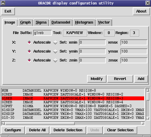
Figure 3: The ORACDISP display configuration tool
The ORAC-DR pipeline has a highly configurable display engine. This note describes how it works and how to use it.
The actual display engine is configured via an ASCII file called disp.dat. A default disp.dat file exists in
the general oracdr distribution (ORAC_DIR). Additionally a default disp.dat is provided by
your instrument scientist or software engineer in the appropriate calibration directory
(ORAC_DATA_CAL)
When you invoke oracdr, the pipeline checks in ORAC_DATA_OUT for an existing disp.dat. If it
does not find one, it copies in the one from ORAC_DATA_CAL, or if that doesn’t exist, the one
from ORAC_DIR. In all of those scenarios you end up with a file in ORAC_DATA_OUT which is
what is used by the display system. Any configuration changes have to be reflected in the
file.
As it is an ASCII file, you may edit the file directly in your favourite editor. However a much easier approach is to type use the oracdisp GUI (simply type oracdisp). This has various options available at the top and shows the disp.dat entries corresponding to those choices at the bottom. Don’t forget to write press the “Configure” button to write the file to disk.
You may use oracdisp (or the editor) to change the display parameters while the pipeline is running.
The disp.dat file has a series of entries consisting of a line each. Each line has a series of space-separated items. All but the first item, the suffix, use the keyword=value syntax.
These items are:
A file suffix representing a particular step of the data reduction process as designated by
that instrument’s file naming convention. For example, for UFTI data “dk” states what to
do with a file called f19990330_00042_dk.sdf. Many entries may be made for a particular
suffix. The following special conventions are used: NUM describes a file ending in just an
observation number (usually representing raw data). For instruments that have multiple
data arrays in a single data frame, S2suffix
(e.g. S2dk) represents the second data array in the frame with the _dk suffix.
A display tool such as Gaia or KAPVIEW (the latter being a collective term for various KAPPA
display tasks). The tools available are determined by the display type (q.v.) selected.
A display type such as graph, image, contour etc. These vary according to the tool selected. The following types are available. The tools which support the given display type are listed in parentheses.
KAPVIEW) Plots a contour plot.
KAPVIEW) Displays data (as points) with a model overlaid.
KAPVIEW, P4) Plots a line graph such as a spectrum.
KAPVIEW) Plots a line graph such as a spectrum.
GAIA, KAPVIEW, P4)
Displays an image.
KAPVIEW) Draws a scatter plot with a Y range of +/- N standard deviations.
KAPVIEW) Displays an image and vectors (e.g. polarimetry data).
For device tools that support it, region addresses the parts of a window where a display ends up. For KAPVIEW, these are: whole screen (0), top left quarter (1), top-right quarter (2), bottom-left quarter (3), bottom-right quarter (4), left half (5), left right (6), top half (7), bottom half (8). Defaults to 0.
The number of the window in which the display is to go. The value of this is simply an identifier and does not presuppose order. If you ask for an image display to go to window 2 and you have configured no displays to go to windows 0 and 1 then you will only get one window on your screen. If you then configure a histogram display to go to window 2 it will go to the same window whereas if you configure it to go to window 1 (or 5 or 9 or anything else besides 2) it will end up in its own window. Note that no windows are launched until they are required.
Specifies whether or not to use a section of the data frame. If set to 1, meaning true, the whole X axis is used. If set to 0, the pixel limits are specified by keywords xmin and xmax. The default is 1.
There are corresponding autoscaling keywords for higher dimensions named yautoscale, 3autoscale, 4autoscale etc.
The X-axis pixel limits of the data to be displayed when xautoscale=1. xmin should be less than or equal to xmax. There are corresponding pixel-range keywords for higher dimensions: ymin and ymax, 3min and 3max, 4min and 4max etc. when autoscaling on the corresponding axis is disabled.
Set to 1 meaning true, this scales this requests that the data are scaled automatically between the data range. In the case of images on GAIA the cut is at the 95 percentile. When zautoscale is 0, the scaling is between the limits defined by keywords zmin and zmax. Defaults to 1 if absent.
When zautoscale is 1, these specifiy the lower and higher scaling limits for the data values.
If the number of dimensions in the data file is greater than that requested, sections in higher dimensions are set to 1 by compressing the undesired dimension(s). Option cut specifies the desired dimension(s).
Option cut is a comma-separated list specifying the dimensionality and axes to retain. The number of entries should equal the dimensionality needed by the type of plot. For instance, a graph only one value is required since a graph is 1-D. The allowed values are X, Y, 3, 4, or 5. If the number of dimensions in the data file is fewer than that requested, ORAC-DR prints a warning message.
Here are two examples, a graph can be displayed from a 2-dimensional image by displaying a cut in the X direction (averaging over the Ys) by setting cut=X. A ‘white-light’ contour plot of a x,y,wavelength spectral data cube may be plotted using cut=X,Y.
There are also parameters special to particular types of display, which also use the keyword=value syntax. These are:
The angle to add to all vectors in a type=vector plot.
The array component to display. Allowed values are Data, Variance, or Error. The default is Data. This applies to type=contour, datamodel, graph, histogram, image, or sigma displays.
The location of the dashed lines for a type=sigma display in standard deviaiton units. This defaults to 3.
If set to 1 (true), error bars are plotted on a type=graph display, provided there is variance information present. The default is 0, meaning do not plot error bars.
This controls the appearance of vectors in a type=vector plot. If set to 0 (false), the default, the vectors are white and have thickness 1. If set to 1 (true), the vectors are yellow with a blue trim and have thickness three.
This is the number of bins to be used for histogram calculation for type=histogram. It defaults to 20.
This specifies the number of contours to plot for type=contour. It defaults to 6 if a non-positive value is supplied.
The standard-deviation range for a type=sigma display. This defaults to 5.
If set to 1 (true), a colour table key is drawn alongside the displayed image. The default is 0, meaning no colour table key is drawn.
Every time a primitive creates a meaningful file with a particular suffix, it sends a display request to
the display system. For example, suppose the primitive that performs dark subtraction creates a frame
called f19990330_00042_dk.sdf and then asks the display system to display it. The display system
consults the disp.dat file for a dk entry. If no such entry is found, the display request is ignored and
nothing happens. If one or more entries are found the display system proceeds to honour the request.
If the disp.dat entry specifies a particular tool and/or window, the display system checks to see if
they exist already and if not, stars them. Then it displays the data with the appropriate
parameters.
Original author: frossie