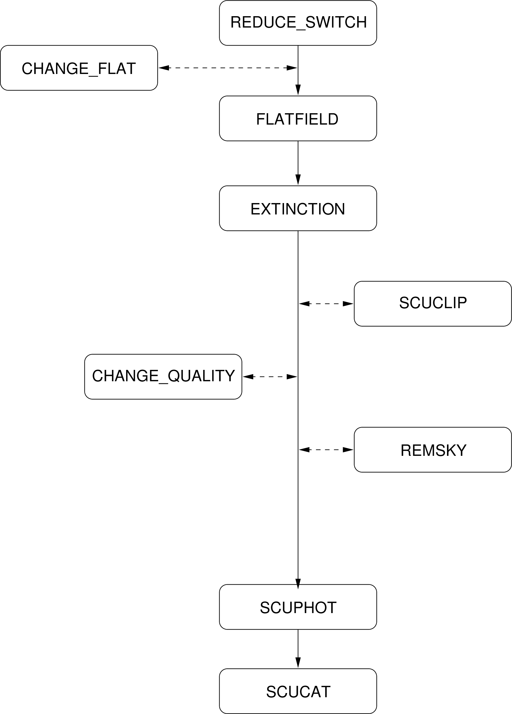
Figure 2: The Surf data reduction flow diagram for PHOTOM data. Optional tasks are
indicated by dashed lines. Note that map data can follow the photometry path and photometry
data can follow the map path if necessary.
The SCUBA transputers take data at a rate of 128 Hz but data are only kept every second (until the high speed data link is installed). Each second of data therefore is the mean of 128 measurements and the standard deviation gives the error. The transputers also detect fast transient spikes which are removed from the calculation of the mean. The number of spikes detected in each measurement is stored for use by the off-line system. Note that the effects of cosmic rays may last significantly longer than 1/128 second and the transputers would probably not detect a spike.
As the SCUBA arrays are not fully-sampled and not on a rectangular grid, images can not be taken in the same way as for an optical CCD array. At least 16 individual secondary mirror, or ‘jiggle’, positions (each of 1 second) are required to make a fully sampled image (64 jiggles are required if both the long and short wave arrays are being used simultaneously). The Surf data reduction package must take these data, combine them and regrid them onto a rectangular grid.
The data-file produced by the on-line system contains all the information necessary to reduce the observations. As well as the raw data, the file contains information on the jiggle pattern, the coordinates of the bolometers relative to the central pixel, flatfield information, internal calibrator signal and general observation parameters.
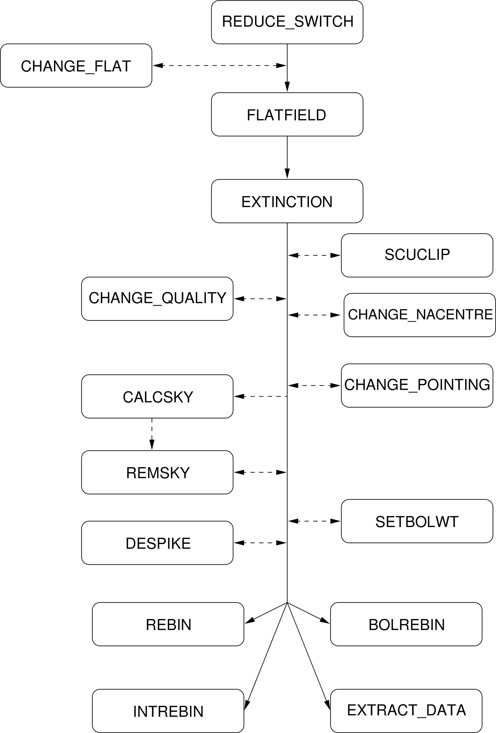
All SCUBA data reduction must include the following stages (see Figs. 2, 3 and 4 for flow diagrams):
The task reduce_switch takes the raw beam switched data and subtracts the off-position from the on-position (‘nods’). If required, this task also divides the data with the internal calibrator signal (this is stored in the demodulated data file as well as the switch information) and sets the level at which spikes detected by the transputers become significant.
The flatfield task takes the output of reduce_switch and flatfields the array by multiplying each bolometer by the volume flatfield value (these are the volumes relative to a reference pixel – the reference bolometers are usually from the array centres: H7 and C14).
The flatfield file itself is actually stored in the demodulated data file. In order to apply a different flatfield, the internal file must be changed with the change_flat task before running flatfield. The change_flat task changes the bolometer positions as well as the volumes. To move flatfield information between files a combination of extract_flat and change_flat should be used.
It is not necessary to flatfield PHOTOM data unless sky removal is to be used or, in some cases, multiple bolometers are to be analysed together.
The extinction task takes the flatfielded data and applies an extinction correction to each pixel one jiggle at a time. The zenith sky opacity (tau) should have been obtained from skydips or estimated from photometry. The optical depth is linearly interpolated as a function of time to find the correction that should be applied to each jiggle.
Since the extinction correction is different for each array, it is at this point that the two arrays must be dealt with independently – the output of this task will contain data for one sub-instrument.
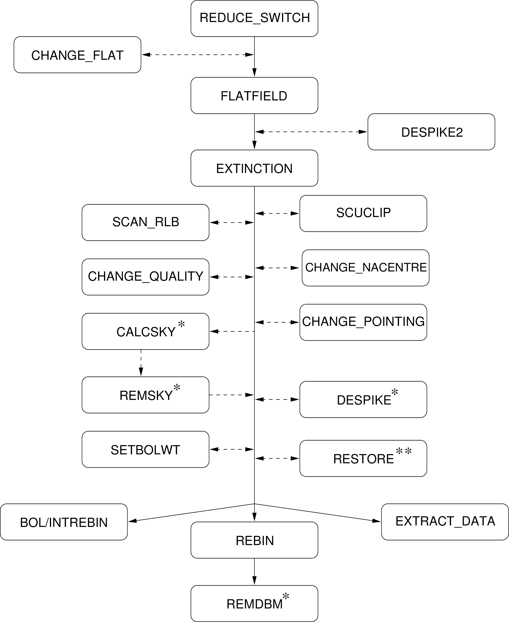
The dual-beam SCAN/MAP data must be restored to a single-beam map at some stage. For data taken whilst chopping along the scan, this is achieved by using the EKH algorithm [11] as implemented in the restore task. In this case the restoration must occur before regridding.
For data taken whilst chopping in a fixed direction on the sky (the so-called “Emerson-II” technique [12]), individual chop configurations must be rebinned independently and then combined using the remdbm task.
In future it is hoped that a maximum entropy algorithm can be implemented [16] for both chopping techniques.
At this stage the data reduction path diverges depending on the observation type. Map data must be regridded onto a rectangular grid using the rebin task (followed by remdbm for SCAN/MAP data if necessary) whereas photometry data must be processed using the scuphot task.
The data reduction process can be automated to a certain extent by using the scuquick script. This script can take as arguments any parameter that is expected by the Surf tasks.
A number of optional tasks are also available:
Tasks are available to change header parameters such as flatfield information (change_flat), applying pointing corrections (change_pointing) or setting pixels (bolometers) and integrations to bad values (change_quality).
Data can be changed using the change_data task. This task can be used to change Data, Variance or Quality arrays and should be used with care.
Instrumental variations and sky-noise can be removed either by using the task remsky (when sky bolometers can be identified) or by using calcsky in combination with remsky (for more complicated sources and scan map data).
Occasionally, spikes get through the transputers and into the demodulated data. Tasks are provided for despiking jiggle/map data (despike), scan/map data (despike2) and photometry data (scuclip8).
Polarimetry observations need to be corrected for instrumental polarisation. The remip task can be used for this.
If the rebinned images are displayed using a program that writes to the AGI graphics database [17], such as Kappa display, the array can be overlaid on the image using the task scuover. This is very useful for identifying noisy bolometers or bad pixels.
The task extract_data is similar to the rebin tasks except that the X, Y and data values are written to an ASCII text file instead of being regridded into a final output image. This is useful for examining the data before regridding (or passing it to an external program for further processing). Obviously this task should not be used to simply examine the data, Kappa tasks such as display and linplot can do that; this task gives you the position of each bolometer in addition to the data value. Additionally, the scuba2mem task can be used for finding the chop positions (although it would then be necessary to use the Convert ndf2ascii task to generate a text file).