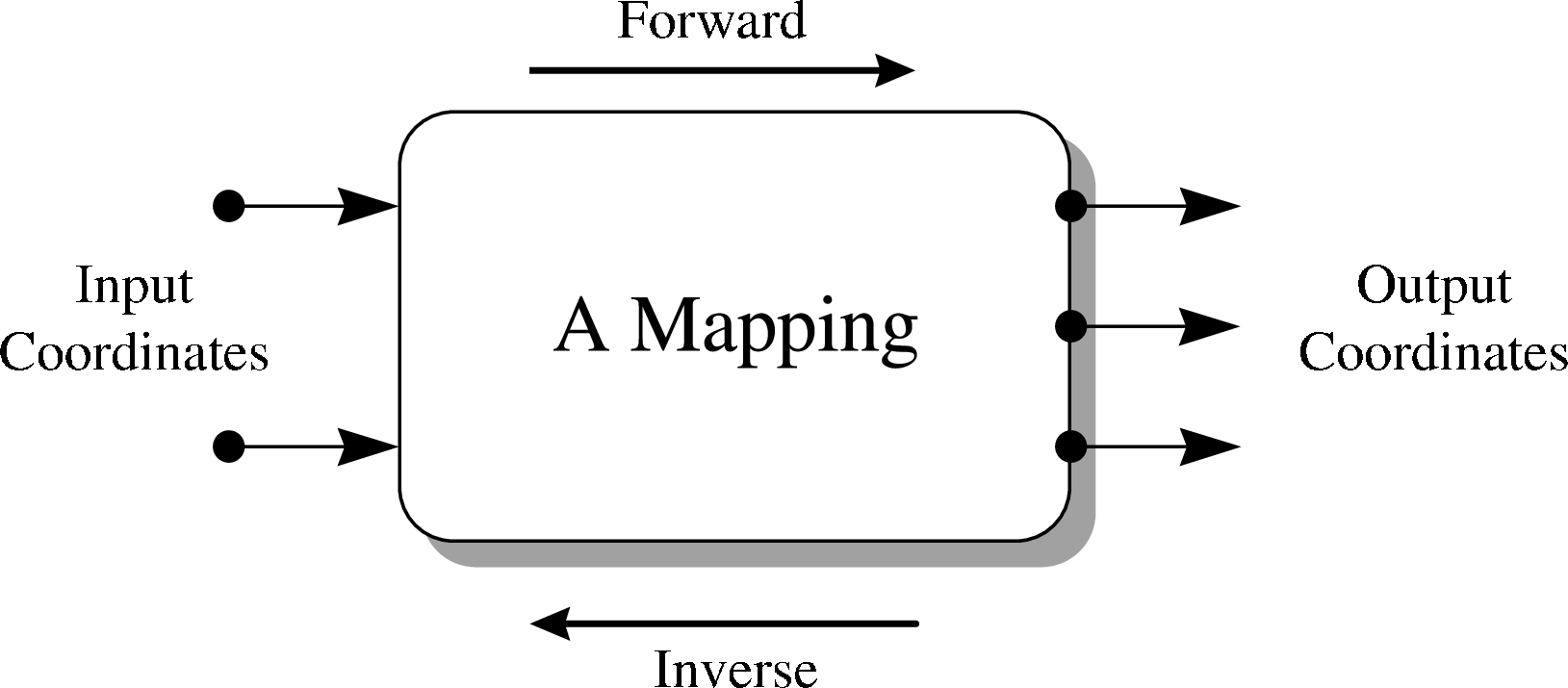
Figure 1: A Mapping viewed as a “black box” for transforming coordinates.
This section presents a brief overview of AST concepts. It is intended as a basic orientation course before you move on to the more technical considerations in subsequent sections.
The relationships between coordinate systems are represented in AST by Objects called Mappings. A Mapping does not represent a coordinate system itself, but merely the process by which you move from one coordinate system to another related one.
A convenient picture of a Mapping is as a “black box” (Figure 1) into which you can feed sets of coordinates.
For each set you feed in, the Mapping returns a corresponding set of transformed coordinates. Since each set of coordinates represents a point in a coordinate space, the Mapping acts to inter-relate corresponding positions in the two spaces, although what these spaces represent is unspecified. Notice that a Mapping need not have the same number of input and output coordinates. That is, the two coordinate spaces which it inter-relates need not have the same number of dimensions.
In many cases, the transformation can, in principle, be performed in either direction: either from the input coordinate space to the output, or vice versa. The first of these is termed the forward transformation and the other the inverse transformation.
Further reading: For a more complete discussion of Mappings, see §5.
The basic concept of a Mapping (§2.1) is rather generic and obviously it is necessary to have specific Mappings that implement specific relationships between coordinate systems. AST provides a range of these, to perform transformations such as the following and, where appropriate, their inverses:
Further reading: For a more complete description of each of the Mappings mentioned above, see its entry in Appendix D. In addition, see the discussion of the PermMap in §5.11, the UnitMap in §5.10 and the IntraMap in §20. The ZoomMap is used as an example throughout §4.
The Mappings described in §2.2 provide a set of basic building blocks from which more complex Mappings may be constructed. The key to doing this is a type of Mapping called a CmpMap, or compound Mapping. A CmpMap’s role is, in principle, very simple: it allows any other pair of Mappings to be joined together into a single entity which behaves as if it were a single Mapping. A CmpMap is therefore a container for another pair of Mappings.
A pair of Mappings may be combined using a CmpMap in either of two ways. The first of these, in series, is illustrated in Figure 2.
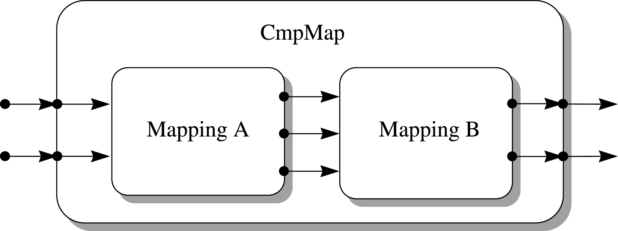
Here, the transformations implemented by each component Mapping are performed one after the other, with the output from the first Mapping feeding into the second. The second way, in parallel, is shown in Figure 3.
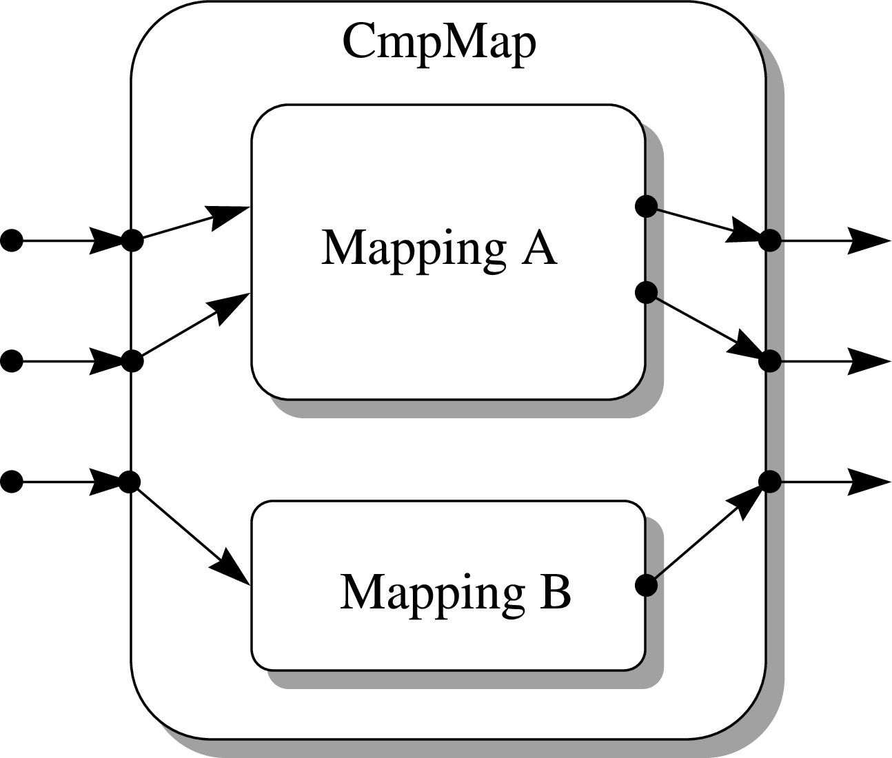
In this case, each Mapping acts on a complementary subset of the input and output coordinates.2
The CmpMap forms the key to building arbitrarily complex Mappings because it is itself a form of Mapping. This means that a CmpMap may contain other CmpMaps as components (e.g. Figure 4). This nesting of CmpMaps can be repeated indefinitely, so that complex Mappings may be built in a hierarchical manner out of simper ones.
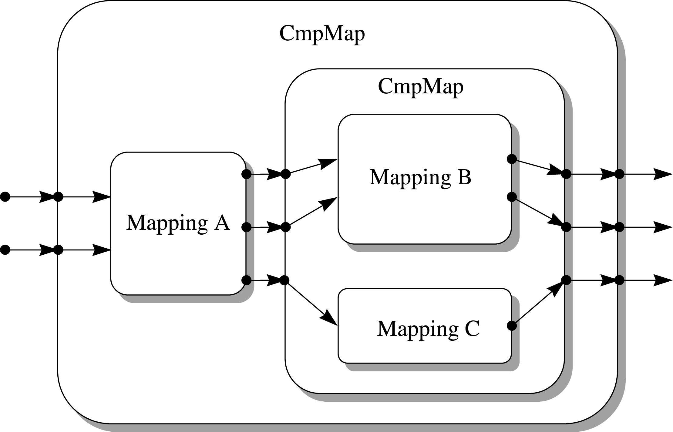
This gives AST great flexibility in the coordinate transformations it can describe.
Further reading: For a more complete description of CmpMaps, see §6. Also see the CmpMap entry in Appendix D.
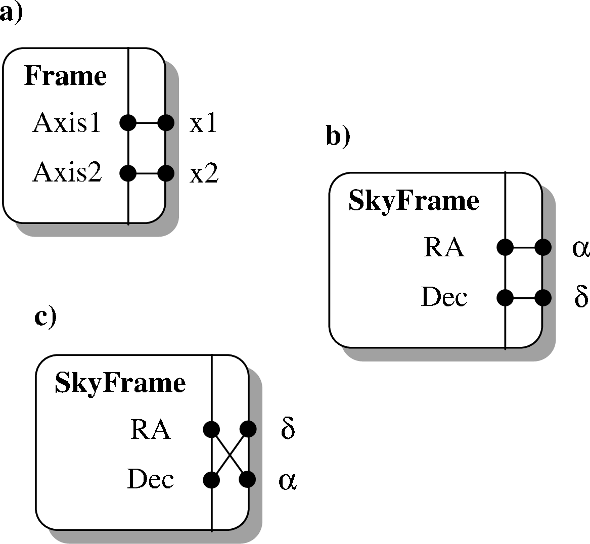
While Mappings (§2.1) represent the relationships between coordinate systems in AST, the coordinate systems themselves are represented by Objects called Frames (Figure 5).
A Frame is similar in concept to the frame you might draw around a graph. It contains information about the labels which appear on the axes, the axis units, a title, knowledge of how to format the coordinate values on each axis, etc. An AST Frame is not, however, restricted to two dimensions and may have any number of axes.
A basic Frame may be used to represent a Cartesian coordinate system by setting values for its attributes (all AST Objects have values associated with them called attributes, which may be set and enquired). Usually, this would involve setting appropriate axis labels and units, for example. Functions are provided for use with Frames to perform operations such as formatting coordinate values as text, calculating distances between points, interchanging axes, etc.
There are several more specialised forms of Frame, which provide the additional functionality required when handling coordinates within some specific physical domain. This ranges from tasks such as formatting axis values, to complex tasks such as determining the transformation between any pair of related coordinate systems. For instance, the SkyFrame (Figure 5b,c), represents celestial coordinate systems, the SpecFrame represents spectral coordinate systems, and the TimeFrame represents time coordinate systems. All these provide a wide range of different systems for describing positions within their associated physical domain, and these may be selected by setting appropriate attributes.
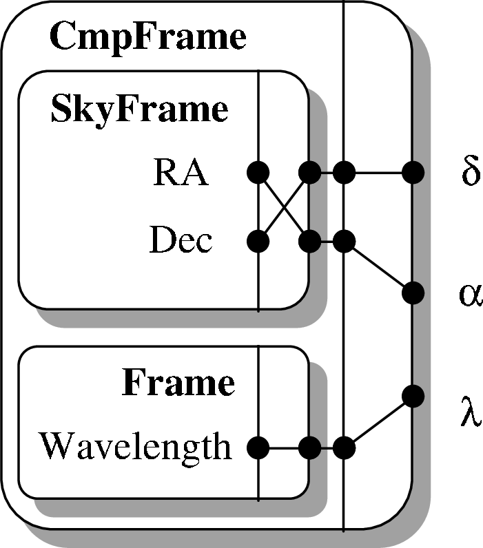
As with compound Mappings (§2.3), it is possible to merge two Frames together to form a compound Frame, or CmpFrame, in which both sets of axes are combined. One could, for example, have celestial coordinates on two axes and an unrelated coordinate (wavelength, perhaps) on a third (Figure 6). Knowledge of the relationships between the axes is preserved internally by the process of constructing the CmpFrame which represents them.
Further reading: For a more complete description of Frames see §7, for SkyFrames see §8 and for SpecFrames see §9. Also see the Frame, SkyFrame, SpecFrame, TimeFrame and CmpFrame entries in Appendix D.
Mappings and Frames may be connected together to form networks called FrameSets, which are used to represent sets of inter-related coordinate systems (Figure 7).
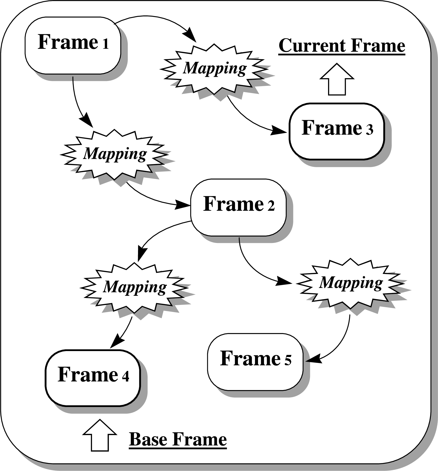
A FrameSet may be extended by adding a new Frame to it, together with an associated Mapping which relates the new coordinate system to one which is already present. This process ensures that there is always exactly one path, via Mappings, between any pair of Frames. A function is provided for identifying this path and returning the complete Mapping.
One of the Frames in a FrameSet is termed its base Frame. This underlies the FrameSet’s purpose, which is to calibrate datasets and other entities by attaching coordinate systems to them. In this context, the base Frame represents the “native” coordinate system (for example, the pixel coordinates of an image). Similarly, one Frame is termed the current Frame and represents the “currently-selected” coordinates. It might, typically, be a celestial or spectral coordinate system and would be used during interactions with a user, as when plotting axes on a graph or producing a table of results. Other Frames within the FrameSet represent a library of alternative coordinate systems which a software user can select by making them current.
Further reading: For a more complete description of FrameSets, see §13 and §14. Also see the FrameSet entry in Appendix D.
AST allows you to convert any kind of Object into a stream of text which contains a full description of that Object. This text may be written out by one program and read back in by another, thus allowing the original Object to be reconstructed.
The filter which converts Objects into text and back again is itself a kind of Object, called a Channel. A Channel provides a number of options for controlling the information content of the text, such as the addition of comments for human interpretation. It is also possible to intercept the text being processed by a Channel so that it may be redirected to/from any chosen external data store, such as a text file, an astronomical dataset, or a network connection.
The text format used by the basic Channel class is peculiar to the AST library - no other software will understand it. However, more specialised forms of Channel are provided which use text formats more widely understood.
To further facilitate the storage of coordinate system information in astronomical datasets, a more specialised form of Channel called a FitsChan is provided. Instead of using free-format text, a FitsChan converts AST Objects to and from FITS header cards. It also allows the information to be encoded in the FITS cards in a number of ways (called encodings), so that WCS information from a variety of sources can be handled.
Another sub-class of Channel, called XmlChan, is a specialised form of Channel that stores the text in the form of XML markup. Currently, two markup formats are provided by the XmlChan class, one is closely related to the text format produced by the basic Channel class (currently, no schema or DTD is available describing this format). The other is a subset of an early draft of the IVOA Space-Time-Coordinates XML (STC-X) schema (V1.20) described at http://www.ivoa.net/Documents/WD/STC/STC-20050225.html3. The version of STC-X that has been adopted by the IVOA differs in several significant respects from V1.20, and therefore this XmlChan format is of historical interest only.
The YamlChan class provides facilities for reading and writing WCS information stored in YAML format using a subset of the the ASDF model developed at StSci (see http://asdf-standard.readthedocs.io).
Finally, the StcsChan class provides facilities for reading and writing IVOA STC-S region descriptions. STC-S (see http://www.ivoa.net/Documents/latest/STC-S.html) is a linear string syntax that allows simple specification of STC metadata. AST supports a subset of the STC-S specification, allowing an STC-S description of a region within an AST-supported astronomical coordinate system to be converted into an equivalent AST Region object, and vice-versa.
Further reading: For a more complete description of Channels see §15 and for FitsChans see §16 and §17. Also see the Channel and FitsChan entries in Appendix D and the Encoding entry in Appendix C.
Two dimensional graphical output is supported by a specialised form of FrameSet called a Plot, whose base Frame corresponds with the native coordinates of the underlying graphics system. Plotting operations are specified in physical coordinates which correspond with the Plot’s current Frame. Typically, this might be a celestial coordinate system.
Three dimensional plotting is also supported, via the Plot3D class - sub-class of Plot.
Operations, such as drawing lines, are automatically transformed from physical to graphical coordinates before plotting, using an adaptive algorithm which ensures smooth curves (because the transformation is usually non-linear). “Missing” coordinates (e.g. graphical coordinates which do not project on to the celestial sphere), discontinuities and generalised clipping are all consistently handled. It is possible, for example, to plot in equatorial coordinates and clip in galactic coordinates. The usual plotting operations are provided (text, markers), but a geodesic curve replaces the primitive straight line element. There is also a separate function for drawing axis lines, since these are normally not geodesics.
In addition to drawing coordinate grids over an area of the sky, another common use of the Plot class is to produce line plots such as flux against wavelength, displacement again time, etc. For these situations the current Frame of the Plot would be a compound Frame (CmpFrame) containing a pair of 1-dimensional Frames - the first representing the X axis quantity (wavelength, time, etc), and the second representing the Y axis quantity (flux, displacement, etc). The Plot class includes an option for axes to be plotted logarithmically.
Perhaps the most useful graphics function available is for drawing fully annotated coordinate grids (e.g. Figure 8).
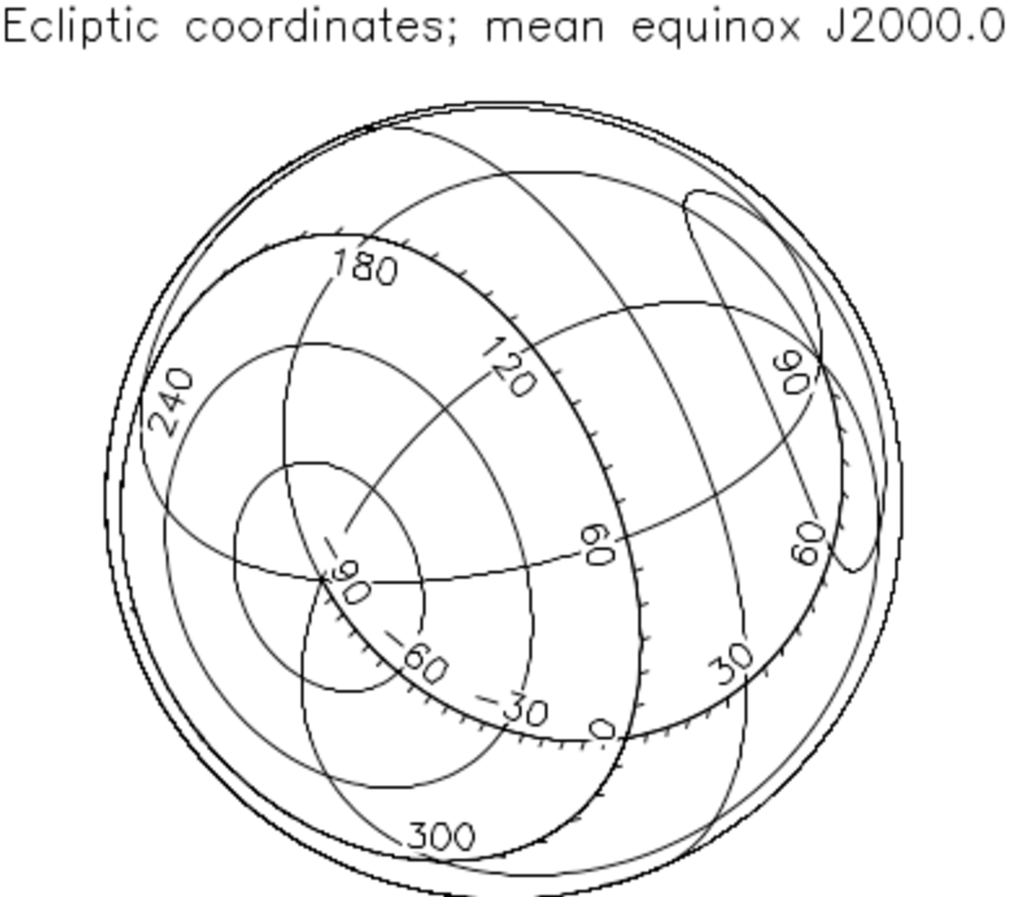
This uses a general algorithm which does not depend on knowledge of the coordinates being represented, so can also handle programmer-defined coordinate systems. Grids for all-sky projections, including polar regions, can be drawn and most aspects of the output (colour, line style, etc.) can be adjusted by setting appropriate Plot attributes.
Further reading: For a more complete description of Plots and how to produce graphical output, see §21. Also see the Plot entry in Appendix D.
2A pair of Mappings can be combined in a third way using a TranMap. A TranMap allows the forward transformation of one Mapping to be combined with the inverse transformation of another to produce a single Mapping.
3XML documents which use only the subset of the STC schema supported by AST can be read by the XmlChan class to produce corresponding AST objects (subclasses of the Stc class). However, the reverse is not possible. That is, AST objects can not currently be written out in the form of STC documents.