4 Dynamic Iterative Map-Making

Rather than cleaning the data by hand and then re-gridding it all at the end, we can instead do everything at once using the Smurf Dynamic Iterative Map-Maker (DIMM).

The DIMM is enabled using the method=iterate switch to the makemap task. In the following example we will produce a map of Uranus using the test data supplied with this Starlink distribution. All of the settings for the DIMM are stored in configuration files. In this example we will use one of the examples that are installed in the Starlink tree, ‘dimmconfig.lis’. For an overview of the different default configuration files available see Section 4.1. The parameters are also fully described in the makemap documentation⁵ or the config files themselves. A local copy can be made and altered if desired. 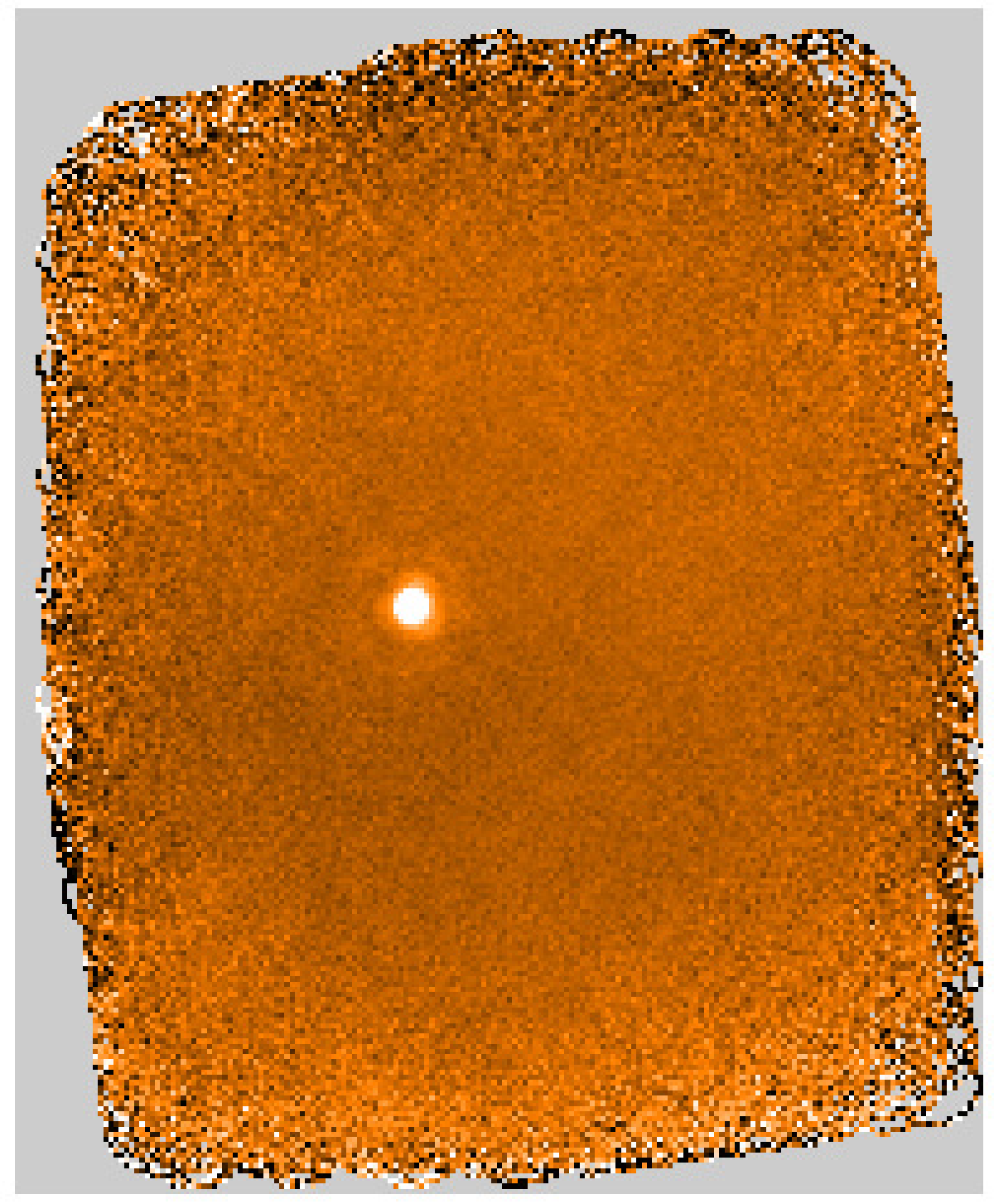The following command invokes the DIMM to produce the image shown in Fig. 9 with 2 arcsec pixels:

This excerpt shows the initial output of the DIMM. Note that the basic dimensions of the data being processed are listed near the start of the first iteration, as well as the QUALITY flagging statistics. This report is similar to that produced by the Kappa task showqual in Section 3.7. At the beginning, the main purpose is to indicate how many bolometers are being used: 368 bolometers were turned off during data acquisition (BADDA); and 40 bolometers exceeded the acceptable noise threshold (NOISE). There were also small numbers of samples flagged as containing spikes and jumps. The total number of bad bolometers (BADBOL) is 413. Accounting for these, and the small numbers of additionally flagged samples, $866.916$ effective bolometers are available at the start of the first iteration.

After each subsequent iteration a new QUALITY report is produced, indicating how the flags have changed. An important flag that appears in the QUALITY report following the first iteration is COM: the DIMM rejects bolometers (or portions of their time series) if they differ significantly from the common-mode (average) of the remaining bolometers. Another useful quantity reported is CHISQUARED – the RMS of the residual (time series with the various model components removed) for all of the samples with good QUALITY, normalized by the measured white noise levels.

This particular configuration executes a maximum of 5 iterations, but stops sooner if the change in CHISQUARED is less then 0.001. In this case, it reaches this stopping criterion after 5 iterations:

Note that compared to the initial report, the total number of samples with good QUALITY (Total samples available for map) has dropped from 10402995 to 10010475 (about a 4 per cent decrease) as additional samples were flagged in each iteration.

Figure 9: Map of Uranus produced with the Smurf task makemap using the iterative algorithm with default parameters. The S/N of the source is now greatly improved compared to the simplistic reduction in Fig. 7, and the negative ringing has been removed.

The iterative map-maker estimates several components of the bolometer signal in addition to the astronomical signal that goes into the map. The particular sequence of components that it fits is specified by modelorder in the configuration file. All of the examples provided with Smurf are derived from $STARLINK_DIR/share/smurf/dimmconfig.lis, and we show the relevant excerpt here:

By default, the final values of these fitted models are not written to files. However, this can be modified by setting exportndf in the configuration file to the list of models that you wish to view:

If we make a local copy of dimmconfig.lis, add the above exportndf line, and re-run the iterative map-maker with this modified configuration, it now produces several new files at the end:

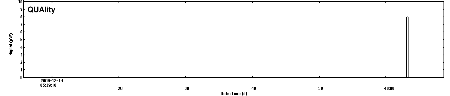
Note that the quality and variance for the data are stored as the VARIANCE and QUALITY components within the residual file NDF.

As with the input data, these are all standard Starlink NDF files which can be examined using all of the existing tools, and can be used by other Smurf routines such as sc2clean, sc2fft, and makemap. The base of the filenames is the first input file that went into the maps for each subarray, and the ‘con’ suffix indicates that several data files may have been concatenated together. The new files are: ‘*ast.sdf’, the time-domain projection of the astronomical signal as estimated in the final map (same dimensions as the input bolometer data); ‘*com.sdf’, an estimate of the common-mode signal (predominantly sky emission and fridge temperature variations); ‘*flt.sdf’, additional noise (low-frequency noise in this particular case) that was filtered out of each bolometer (same dimensions as the input bolometer data); and finally ‘*res.sdf’, the residual bolometer signal once the other components have been subtracted from the original data, which should look predominantly like white noise (again, same dimensions as the input bolometer data).

Figure 10: Time-domain components of the iterative solution for bolometer (13,23). From top to bottom: ASTronomical signal (clearly showing Uranus as positive spikes); COMmon mode (dominated by 30 s fridge variations); FiLTered (residual low-frequency noise missed by COM); RESidual (looking flat, except for a small residual around the location of a repaired DC step); and QUAlity (indicating the location of the DC step – the numerical value 8; this region of the data is not used in the final map). All of the plots were produced with Gaia, restricting the range of the $x$-axis to samples 2840–11500.

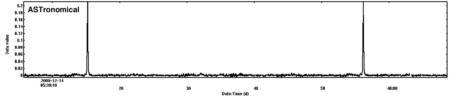
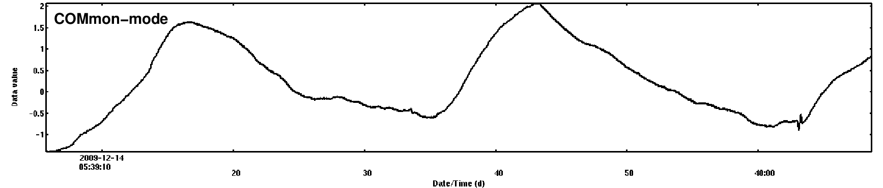
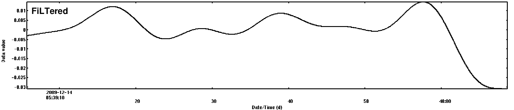
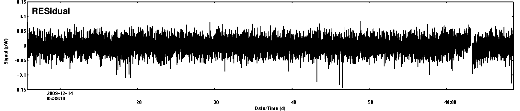
Time traces for a single bolometer are compared for all of these model components in Fig. 10. Uranus is clearly seen as a positive spike in the astronomical signal component. The common-mode signal is the next largest, clearly exhibiting the 30 s fridge variations that are apparent in the raw data. The residual noise removed by the high-pass filter is significant, but much smaller than the common-mode component. Finally, the residual signal is quite flat, indicating that most of the signal has been accounted for in the other model components.

4.1 Configuration Files

Since the DIMM has a large number of parameters, several configuration files are supplied with Smurf for reducing common types of data. All of these files can be found in
$STARLINK_DIR/share/smurf/ with filenames of the form dimmconfig*.lis. The default dimmconfig.lis should give reasonable results for most observations. Note that this file also contains the full set of parameters with extensive documentation. For clarity, all of the other configuration files for specific observations types are derived from dimmconfig.lis and simply override the relevant parameters.

While we have tested a wide variety of data sets with these files, it is certainly worth trying at least the default, and the specific configuration that sounds like it would be appropriate for your project:

dimmconfig.lis

Before the iterative solution begins, some pre-processing steps are performed, like repairing DC steps, turning off particularly noisy bolometers (see the
noiseclip parameter), and the mean levels are subtracted. This default configuration solves for the following models: COM, GAI, EXT, FLT, AST, NOI. The components COM and GAI work together to calculate the average signal template of all the bolometers, and then fit/remove the templates from each bolometer. They also identify outlier bolometers that do not resemble the template and remove them from the final solution. The component EXT applies the extinction correction (derived from the water-vapour radiometer by default), and then FLT applies a high-pass filter to the data, above frequencies that correspond to angular scales of 600 arcsec and 300 arcsec at 450 $\mu$m and 850 $\mu$m, respectively (as established automatically from the mean slew speed of the scan). These cutoff frequencies were chosen through trial and error, but appear to give good results under a wide variety of situations. Finally, AST estimates the astronomical signal contribution to the bolometer signals from the current map estimate, and NOI measures the noise in the residual signals for each bolometer to establish weights for the data as they are placed into the map in subsequent iterations.

dimmconfig_blank_field.lis

This configuration is tuned for deep surveys for which the goal is to detect low-S/N point sources. Instead of iteratively applying a high-pass filter (FLT), which can result in convergence problems when there is little signal in the map, a single, harsher high-pass filter is applied as a pre-processing step (corresponding to 200 arcsec scales at both 450 $\mu$m and 850 $\mu$m). There are also more conservative cuts to remove noisy/problematic bolometers. Finally, the parameters ast.zero_lowhits and ast.zero_notlast are set to constrain much of the map to precisely zero for all but the last of 5 iterations. This helps with map convergence, and is a reasonable prior for a blank-field. Normally the map would then be processed using a matched filter (see Section 6.1).

dimmconfig_bright.lis

This configuration is aimed at reducing maps of bright sources. Weaker noise clipping, DC step thresholds and common-mode rejection are used. In addition, the number of iterations is increased to a fixed value of 20 to allow potentially large-scale structures to converge.

dimmconfig_bright_compact.lis

This configuration is aimed at reducing maps of bright, compact sources that are isolated at the centre of the map, and is derived from dimmconfig_bright.lis. The addition of ast.zero_circle and ast.zero_notlast parameters are used to constrain the map to zero beyond a radius of 1 arcmin for all but the final iteration. This strategy helps with map convergence significantly, and can provide good maps of bright sources, even in cases where scan patterns failed and the telescope degenerated into scanning back-and-forth along a single position angle on the sky.

dimmconfig_bright_extended.lis

This configuration is for reducing maps of bright extended sources, and is also derived from dimmconfig_bright.lis. Here ast.zero_snr is used to constrain the map to zero wherever the S/N is lower than 5-$\sigma$. We recommend setting the parameter itermap=1, and then visually inspecting the maps produced after each iteration (e.g., gaia map.more.smurf.itermaps) to help determine an appropriate number of iterations.

If you want to modify parameters for a particular config file the best approach is to create a new file and first include a directive to load the file you want to modify and then supply your own parameters. You can see this technique is used in the installed configuration files to reference them all to dimmconfig.lis.