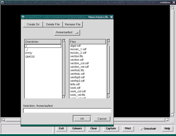
Figure 20: An XDialog script based on velmap; here it asks for an input file.
csh scriptsAn excellent introduction to writing csh scripts can be found in the C-shell Cookbook
(SC/4).
Seemingly a trivial problem with a simple solution this turns out to be slightly more complicated than you would initially expect. Presuming we need an integer pixel position to give to another application we are using in our script, we can use the following code block to do so.
Here we run the cursor application, requesting it to return co-ordinates in the PIXEL Frame, creating a lock file to stop further execution of the script until the user has clicked on the graphics display window. We then delete the lock file and retrieve the cursor position using parget. cursor returns each co-ordinates as a floating-point value, whereas we require an integer pixel index. We therefore use calc to convert from co-ordinates to indices by adding 0.5 and finding the nearest integer.
This functionality has been encapsulated within the script $DATACUBE_DIR/getcurpos.csh.
A similar, but slightly easier, problem is to grab real world co-ordinates from a cursor click on a graphics display window.
Here we run the cursor application, again creating a lock file to stop further execution of the script. We then delete the lock file and retrieve the cursor position using parget.
This functionality has been encapsulated within the script $DATACUBE_DIR/getcurpos.csh.
The following code will overplot the contours of one dataset on to the greyscale image of another of the same spatial size using the Kappa display and contour tasks.
This is useful in many circumstances, for instance, plotting the contours of a white-light image over a passband image, or velocity map.
If you want to make use of the bc utility to carry out floating-point calculations in csh scripts you
may come across a problem with scientific notation. In many cases applications return
scientific notation in the form 3.0E+08, or 3.0E-0.8, while bc requires these numbers to
be of the form 3.0*10^08, or 3.0*10^-08. The following example segment of code takes
two numbers in the first format and passes them to bc in the correct manner so that it can
do some arithmetic with them. bc will return a floating-point number (not in scientific
notation).
The scale specifies the number of decimal places.
An alternative to using bc inside your scripts is the Kappa calc command which can evaluate many arbitrary mathematical expressions, as in this extract.
here we evaluate the Doppler velocity of an emission line using three calls to calc, although the velocity could have been derived in a single expression.
You may need to access information that was contained in the FITS header to carry out your data analysis, having converted your data to NDF format to make use of the Starlink software the FITS header keywords are still accessible as part of an NDF extension. Kappa has a number of tools specifically written to handle FITS keywords (see SUN/95 for details).
The recommended way to find the value of a FITS header keyword is by using the fitsval application.
For instance, you could obtain the value of the FITS keyword CRVAL3 (see Section 4.3) as
follows.
This could be used in a script to take appropriate action along with other Kappa FITS manipulation tools.
Here we use Kappa fitsexist comtmnd to check that the the keyword we are interested in exists, then the fitsval command to query its value and act on the information.
If it possible to build an NDF file from a flat ASCII text file using the Convert application ascii2ndf and then use Kappa and Datacube applications to modify the structure and contents of the NDF extensions until it has the correct specifications.
Here we take a flat ASCII data file $datfile and create an NDF of dimensions $dims[1]
$dims[2],
with data type _DOUBLE, using ascii2ndf. We then cal upon setmagic to flag all pixels that have the
value
in the NDF with the standard bad ‘magic’ value, in this case VAL__BADD. setorigin sets the pixel origin
to ($lbnd[1],$lbnd[2]). We then use ascii2ndf again to attach a variance array, from the ASCII flat
file $varfile, to our newly created NDF.
For both invocations of ascii2ndf we make use of the MAXLEN parameter. This is the maximum record
length (in bytes) of the records within the input text file, the default value being 512. If you
attempt to generate an NDF from a file where many of the entries are double-precision
numbers, it might be necessary to set this value higher than the default value otherwise some
records (lines) may become truncated leading to ‘stepping’ effects within your output
NDF.
After including our variance array, we attach AXIS information using the setaxis application, and
incorporate WCS information with wcscopy application, both from Kappa. We clone this information
from an NDF whose world co-ordinate information is the same as our newly created NDF. If we
wanted to avoid copying the AXIS information (or if the NDF from where we were cloning had no
WCS information) we could make use of the wcscopy command’s TR parameter to provide a
transformation matrix.
Alternatively, we could make use of the Kappa setaxis command to create an AXIS structure within the NDF being cloned obtained from its existing WCS extension via the $likefile parameter. setaxis should be invoked for each axis. Then we copying the AXIS and WCS structures to our new NDF.
The above usage of setaxis is sometimes needed when including non-WCS compliant legacy applications, such as fitgauss, in scripts, as these legacy tasks do recognise the AXIS structure.
The Xdialog program is designed as a drop-in replacement for the dialog and cdialog programs. It can convert a simple terminal based script into a program with an X-Windows (GUI) interface. The requirements to install XDialog is that you must have the X11 libraries and GTK+ libraries (version 1.2.) installed on your machine. GTK+ comes installed by default with most recent Linux distributions (being necessary to run the GNOME desktop), however, it can be compiled under both Solaris and Tru64 UNIX, and with the adoption of GNOME as the standard SUN desktop will increasing come installed by default on platforms other than Linux.
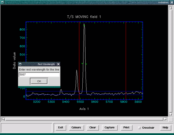
Most shell scripts are easily converted to use Xdialog, for example we quickly modified the velmap script to use it, see Figures 20 and 21. More information about XDialog can be found at http://xdialog.dyns.net/.