5 A Fuller Reduction: Removing bad bolometers, sky-noise and spikes
5.1 Identifying and Blanking Noisy Bolometers
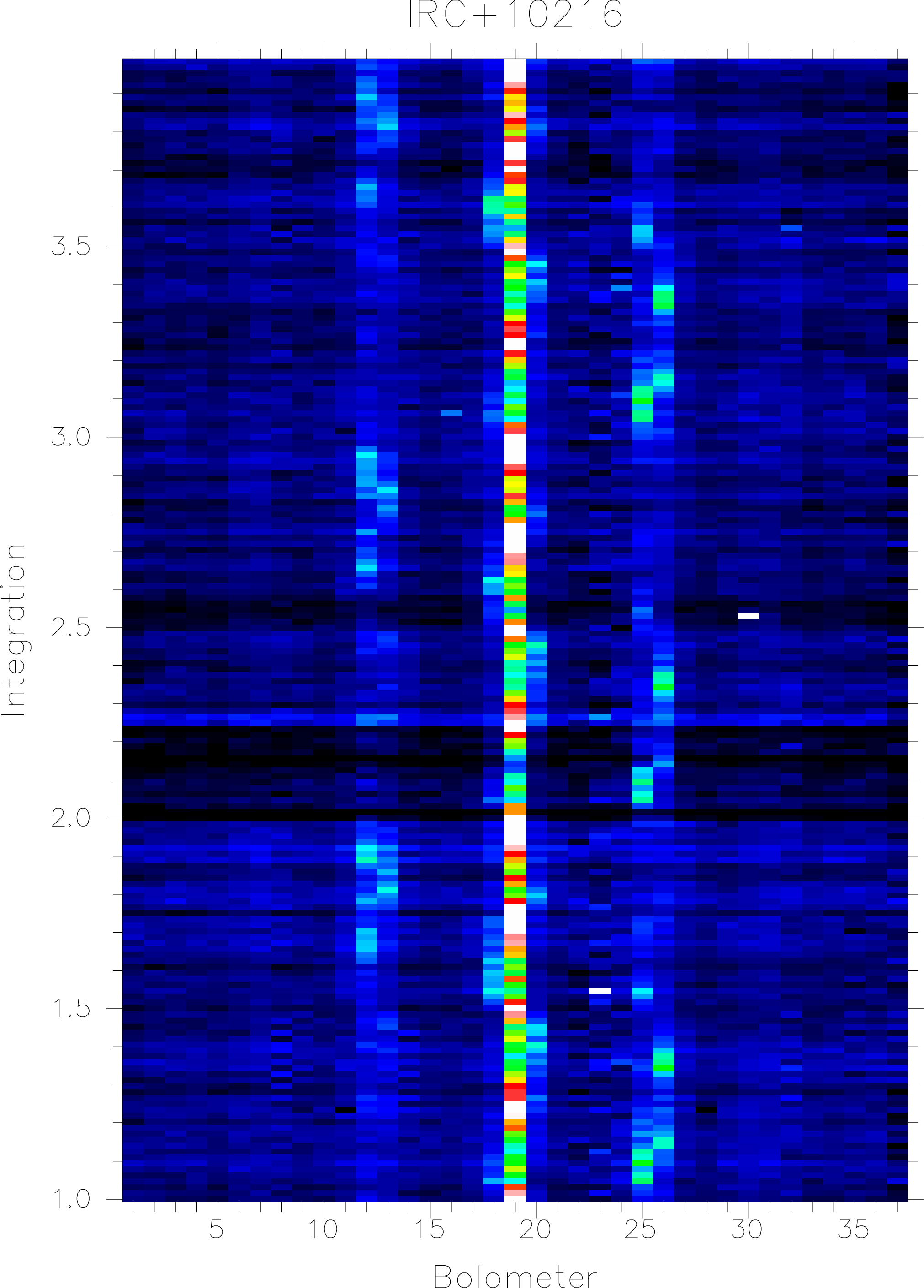
From the plot shown in Fig. 2 we can see that the map suffers from some sky noise, e.g. visible as the
dark striping at the beginning of integration 2. The central bolometer, 19 (h7) shows a clear signal, and
we do not see any really bad (noisy) bolometers, except perhaps bolometer 23. Even so, we first need
to blank out bad bolometers. There are several ways to identify bad bolometers. The easiest
way, although it may not pick up all noisy bolometers for your particular map, is to run
scunoise, which is a GUI that allows you to plot and identify all noisy bolometers using noise
measurements done during the run. If we do this for the night of 19971208 we find a total
of 9 noise measurements and we can see that some bolometers come and go, but 23 is
always noisy. From the most nearby noise measurement, #88, we find that 23, 32 and 37 have
noise levels above 100 nV and 12 is also about twice as noisy as the majority of the array,
which should have a noise level around 40 nV. Before we set these bolometers to bad we
plot the bolometers with mlinplot to check that these bolometers are indeed noisy in our
map.
% mlinplot i86_lon_ext absaxs=2 lnindx=’21:32’
YLIMIT - Vertical display limits /[-0.002588027,0.09385466]/ >
DEVICE - Name of display device /@xwindows/ >
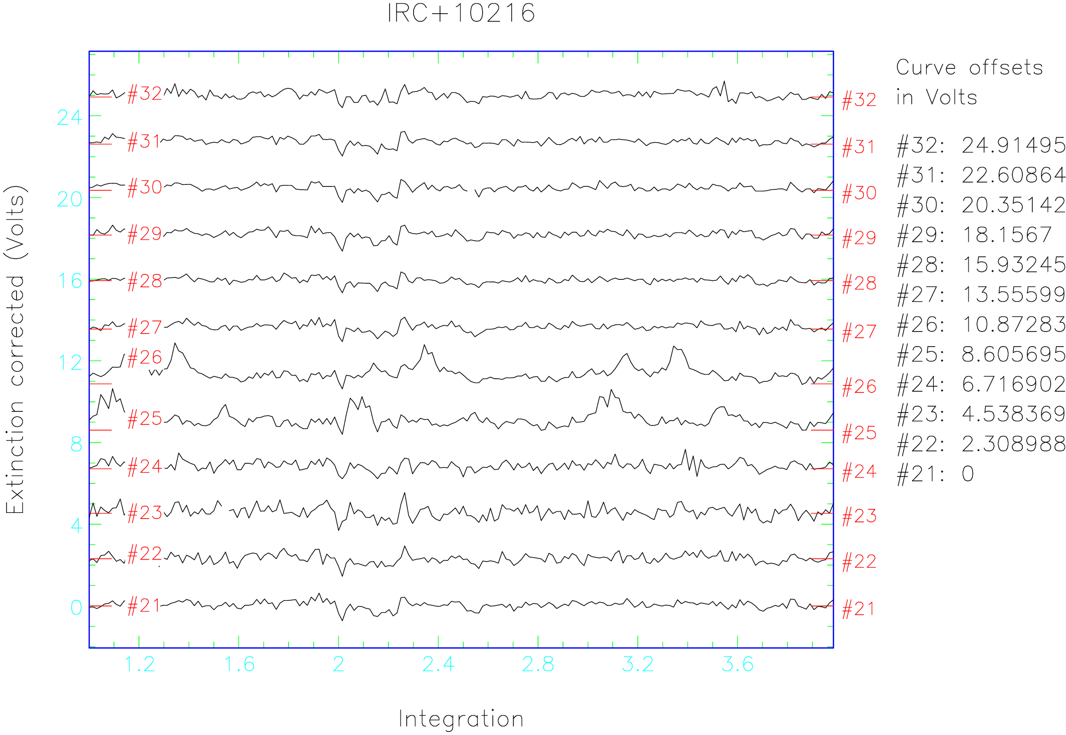
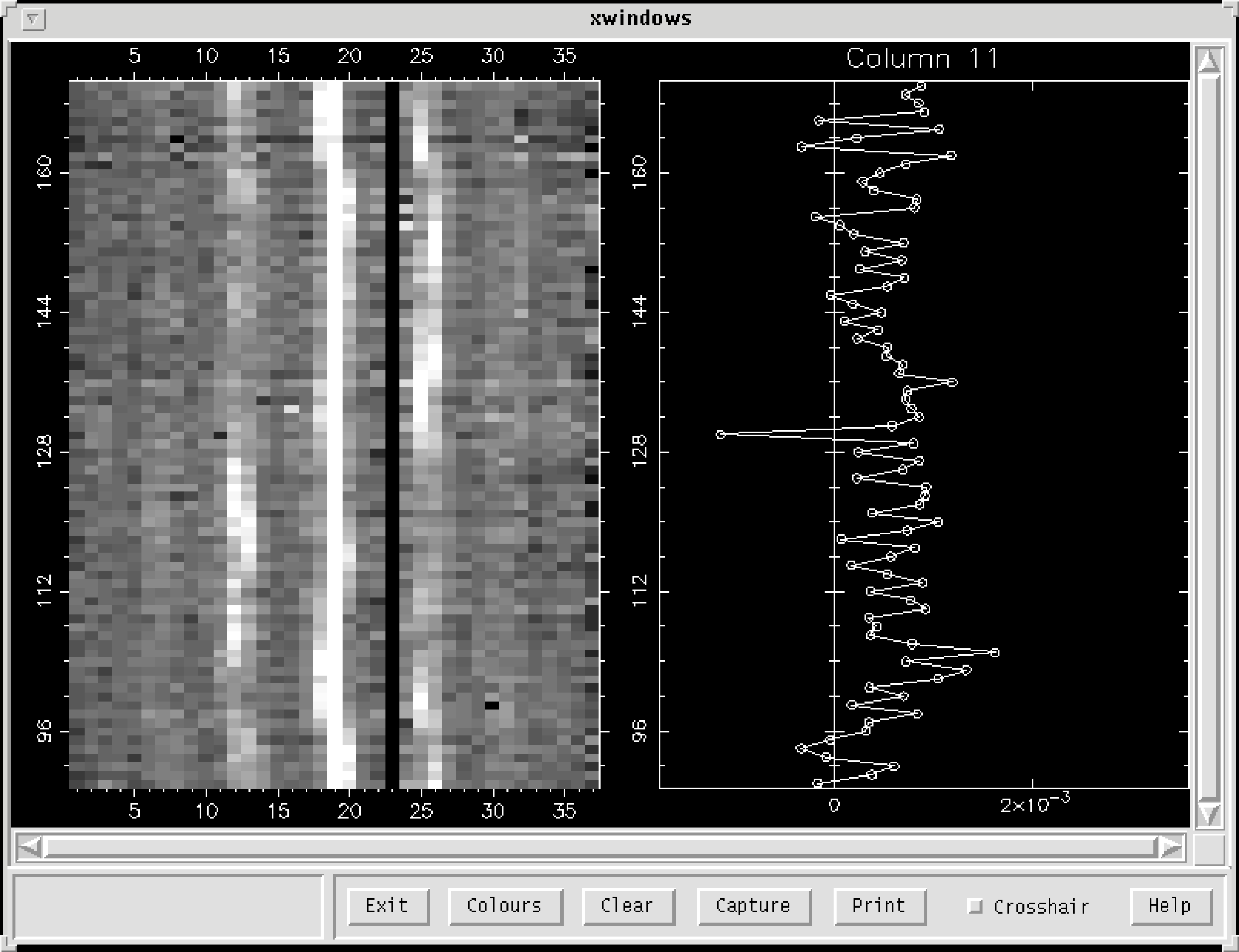
In the above example the bolometers 21 – 32 are plotted as a function of integration time (Fig. 3).
Bolometer 23 is indeed the noisiest pixel, but 22, and 24 are noisy as well and actually
worse than 32, which was picked up by scunoise. Fig. 3 shows strong sky noise, which
makes it difficult to see the true noise level of the bolometers, and it is often wise to do a
sky noise reduction (see below), so that one can more easily identify noisy bolometers.
Go through the whole array by choosing suitable bolometer ranges with the parameter
lnindx. In this example we choose to only blank out bolometer 23, which we set to bad
using change_quality. Bolometers 8 and 14 also appear noisy, more so than 12, which we
picked up in the noise measurement, but for the time being we let them stay. When we
go through the bolometers with mlinplot we can also see a few spikes, which we will
deal with shortly. Let us now set bolometer 23 with change_quality. Note that we need
to surround the file name with both single and double quotes if we list more than one
bolometer.
% change_quality "’i86_lon_ext{b23}’"
SURF: run 86 was a MAP observation of IRC+10216
SURF: file has data for 37 bolometers, measured at 192 positions.
- there are data for 4 exposure(s) in 3 integration(s) in 1
measurements.
BAD_QUALITY - Set quality to bad? (No will set quality to good) /YES/
>
5.2 Initial sky noise removal
As we have already seen, sky noise can be a dominant noise source in a map, but as long as
the sky noise is correlated over the array, it can be removed. One can do this in several
different ways, but for a single short integration map one will always use remsky. In the
automated SCUBA reduction Jenness et al. [14] use the median option in remsky and
include all bolometers. Since we have a centrally symmetric source, we take the second
ring, r2, of bolometers using the median option to avoid spikes that may be present in the
data.
% remsky
IN - Name of input file containing demodulated map data
/@o86_lon_ext/ >
SURF: run 86 was a MAP observation with JIGGLE sampling of object
IRC+10216
OUT - Name of output file /’o86_lon_sky’/ >
BOLOMETERS - The Sky bolometers, [a1,a2] for an array
/[’4’,’9’,’29’]/ > r2
SURF: Using 12 sky bolometers
MODE - Sky removal mode /’median’/ >
Sky noise: 0.000602097 (192 points)
Adding mean background level back onto data (value=0.0003676229)
Note that the default behavior of this routine is to add the mean bolometer signal back in to data (this
may not be what you wish to do) if it’s not then type:
5.3 Initial Despiking
Let us now remove the worst spikes by using the Surf task scuclip to take out any spikes exceeding 5
sigma.
% scuclip
IN - Name of input file containing demodulated map data
/@i86_lon_sky/ >
SURF: run 86 was a MAP observation with JIGGLE sampling of object
IRC+10216
OUT - Name of output file /’i86_lon_clip’/ >
NSIGMA - How many sigma to despike bolometers /5/ >
SURF: Removed 3 spikes
scuclip removed 3 spikes in the data, which will do for the moment.
Following despiking and sky removal one can then run rebin. The process of sky removal will
significantly improve any maps which have a ‘tiled’ pattern due to varying sky emission between the
two switch positions. Below we discuss in more detail how to most efficiently remove sky noise,
which depends on what data sets we have.
5.4 Sky noise removal (a)- remsky.
In Section 5.2 we already used remsky to remove sky noise by choosing a ring of bolometers around
the center and we could even have used all bolometers in the array. However, for short chop throws,
or where we have an extended source or where the source is not centered in the array one should be
more careful. A good way to identify suitable sky bolometers (i.e. bolometers without any source
emission) is to convert the map into Az/El (assuming we chopped in Az) so that we can identify
bolometers at the edge of the array, which are not affected by the chop nor by any source emission.
We regrid the extinction corrected data with the Surf task rebin, setting the parameter
to az. In the example below we use the same data set on
IRC10216
as we used before. We plot the map immediately with display using the option faint and
overlay the bolometer array using scuover (use noname if you want the bolometers as
numbers).
% display axes clear
IN - NDF to be displayed /@i86_lon_reb/ >
DEVICE - Name of display device /@epsfcol_p/ > xwindows
MODE - Method to define the scaling limits /’fa’/ >
Data will be scaled from -0.0012709096772596 to 0.013754481449723.
% scuover
DEVICE - Name of graphics device /@xwindows/ >
Current picture has name: DATA, comment: KAPPA_DISPLAY.
Using /home/sandell/dec8/i86_lon_reb as the input NDF.
SURF: file contains data for 4 exposure(s) in 3 integration(s) in 1
measurement(s)
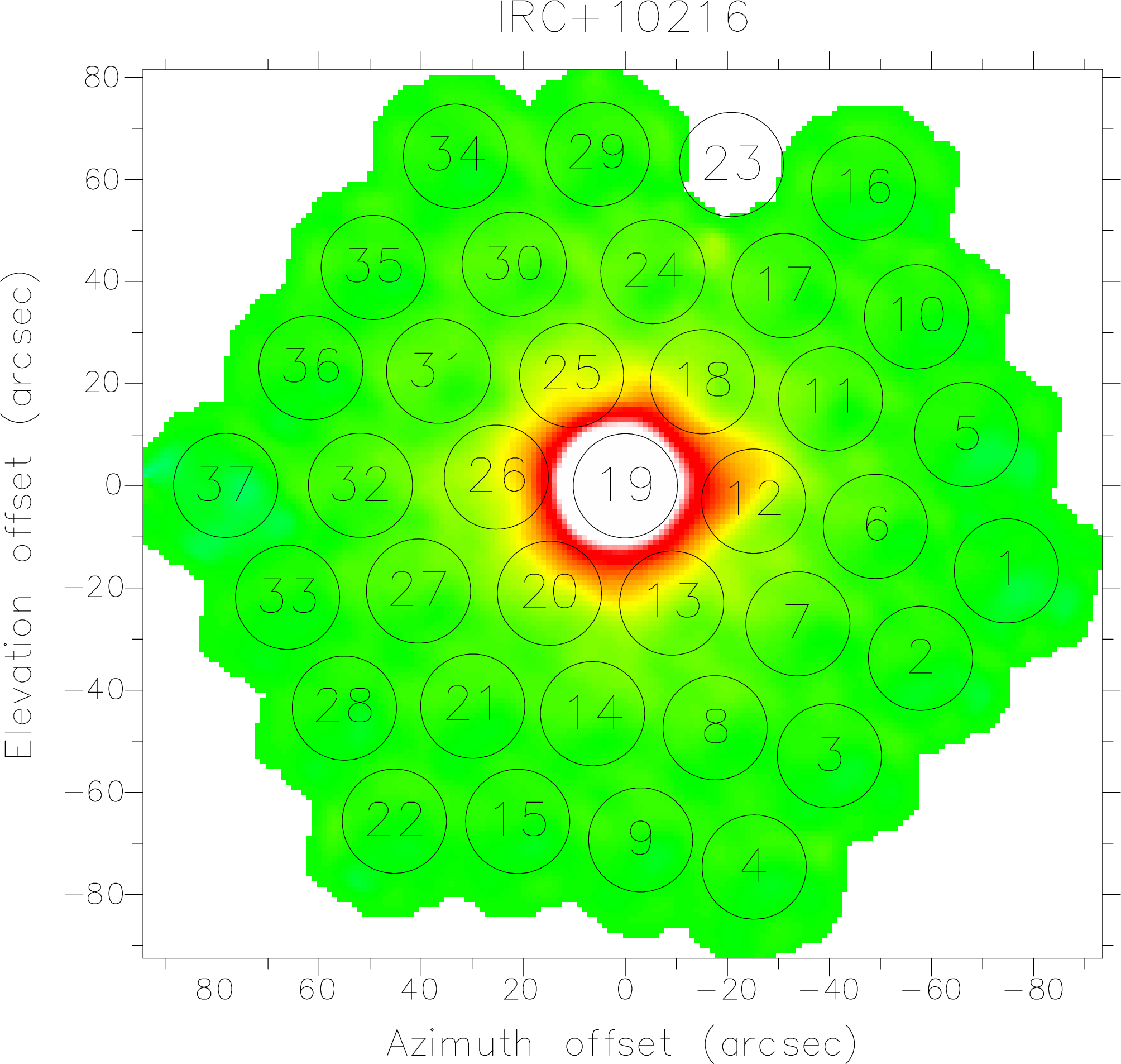
IRC10216 is
extended at 850m,
because of its large CO envelope, and we therefore want to use edge pixels away from the
chop direction (usually az) to avoid removing any real signal from the data. In our map of
IRC+10216 (Fig. 4) one would therefore take bolometers 4,9,15 and 22 in the south and
16, 29, and 34 in the north. If we now run remsky on the extinction corrected data, we
notice that the background level added back to the map was lower than when we used
ring 2, which therefore picks up some of the faint extended emission surrounding
IRC10216.
% remsky
IN - Name of input file containing demodulated map data
/@o86_lon_sky/ > o86_lon
_ext
SURF: run 86 was a MAP observation with JIGGLE sampling of object
IRC+10216
OUT - Name of output file /’i86_lon_sky’/ >
BOLOMETERS - The Sky bolometers, [a1,a2] for an array /’r2’/ >
[4,9,15,16,29,34]
SURF: Using 6 sky bolometers
MODE - Sky removal mode /’median’/ >
Sky noise: 0.0005996103 (192 points)
Adding mean background level back onto data (value=6.3598651E-5)
5.5 Sky noise removal (b)- calcsky
Quite often, especially when we observe galactic sources embedded in dark or molecular cloud, it is
impossible to find any bolometers that do not pick up source emission. As long as the
source emission is relatively smooth, this will only affect the mean level in the map, and
any base level that gets removed with remsky can be added back into the image using
. But, if
there is structure in the source emission over our sky bolometers, these variations will be
interpreted as sky noise and therefore affect the morphology of our map. For extended
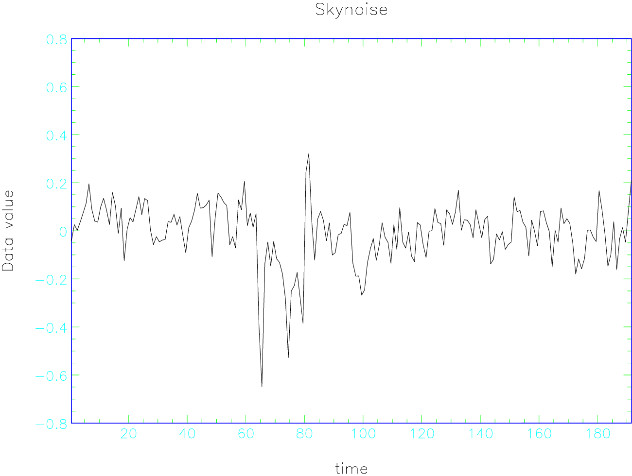
sources we should therefore use calcsky. The task calcsky computes a model of the source,
which it then subtracts from each bolometer to give an estimate of the sky variation, which
is put into the file extension .more.reds.sky, which can be examined with e.g. linplot,
e.g.,
% linplot i86_lon_cal.more.reds.sky device=xwindows
shows the computed sky noise variations for the scan 86, that we will re-analyze below
(Fig. 5).
We can improve the model by adding data sets to calcsky the same way as we use rebin for
coadding data. If one has already produced a final map of the source, one can use this
map as the input model for calcsky. For multiple data sets we should make an input file
with weights and offsets as we do for rebin, see Section 5.8. We now choose the default
model, which will be the median of all the observed maps. Once calcsky is done, we go
back and run remsky on each data file which was included in the model computed by
calcsky.
calcsky works extremely well even for extended sources, if one has kept the chop
position fixed. For extended sources it is therefore an advantage to chop in a fixed
ra/dec frame. One can also use calcsky for a spherically symmetric source like
IRC10216
even for a chop throw of 60”, but then one should use az option for the
.
calcsky also includes the option to account for the chop throw and direction, and it should
therefore work even when we chop differently on extended emission from one map to the
next.
For scan maps calcsky is our only option for sky noise removal, because in scan maps each bolometer
will normally include both source and sky (see later).
Below we show how to use calcsky on the same file we already reduced with remsky. When we now
run remsky it will not ask for sky bolometers, but will use the sky extension stored in the header to
remove sky noise variations.
% calcsky
OUT_COORDS - Coordinate sys for sky determination /’RJ’/ >
SURF: output coordinates are FK5 J2000.0
REF - Name of first data file to be processed /’i86_lon_sky’/ >
i86_lon_cal
SURF: run 86 was a MAP observation of IRC+10216 with JIGGLE sampling
SURF: file contains data for 4 exposure(s) in 3 integrations(s) in 1
measurement(s)
WEIGHT - Weight to be assigned to input dataset /1/ >
SHIFT_DX - X shift to be applied to input dataset on output map
(arcsec) /0/ >
SHIFT_DY - Y shift to be applied to input dataset on output map
(arcsec) /0/ >
IN - Name of next input file to be processed /!/ >
SURF Input data: (name, weight, dx, dy)
-- 1: i86_lon_cal (1, 0, 0)
BOXSZ - Size of smoothing box (seconds) /2/ >
MODEL - File containing source model /!/ >
% remsky
IN - Name of input file containing demodulated map data
/@i86_lon_ext/ >
SURF: run 86 was a MAP observation with JIGGLE sampling of object
IRC+10216
OUT - Name of output file /’i86_lon_sky’/ > i86_lon_sky
REMSKY: Using SKY extension to determine sky contribution
The sky noise we see in our jiggle maps is due to changes in the sky emission between nods of the
telescope. For unstable sky conditions this results in a tile-pattern in your map. This type of structure
will not be removed by calcsky if we apply it to a single data set. Indeed in this particular example,
remsky with selected sky bolometers gave a much better result than using calcsky. However, for
really extended sources and scan maps we may not have a choice. We will have to use
calcsky followed by remsky.
Another advantage of calcsky which is worth mentioning is that we can run calcsky on the
450m
array and copy the calculated sky noise variations to the
850m array
after appropriate scaling. This enables us to remove sky noise variations on a very faint extended
850m–source,
without subtracting out source emission.
5.6 Manual Despiking
The way we despike jiggle maps depends on whether we have done short or long integrations
and on whether our source is compact or extended. In the above example we only have 3
integrations and despike will miss most spikes. We can still use scuclip but if we want to
go deep, we have to make sure that we don’t clip the source as well. We know that
IRC10216 is
relatively compact with a faint ‘halo’ type emission surrounding the core. It may therefore enough to
use scuclip, but go deeper than in our initial despike effort. To be on the safe side, i.e. to make sure
that we do not clip the source, we set the central bolometer to bad before we start and reset it back to
good afterwards using change_quality.
% change_quality ’i86_lon_sky{b19}’
SURF: run 86 was a MAP observation of IRC+10216
SURF: file has data for 37 bolometers, measured at 192 positions.
- there are data for 4 exposure(s) in 3 integration(s) in 1
measurements.
BAD_QUALITY - Set quality to bad? (No will set quality to good) /YES/
>
% scuclip
IN - Name of input file containing demodulated map data
/@i86_sho_sky/ >
SURF: run 86 was a MAP observation with JIGGLE sampling of object
IRC+10216
OUT - Name of output file /’i86_lon_clip’/ >
NSIGMA - How many sigma to despike bolometers /5/ > 4
SURF: Removed 10 spikes
% change_quality ’i86_lon_clip{b19}’
SURF: run 86 was a MAP observation of IRC+10216
SURF: file has data for 37 bolometers, measured at 192 positions.
- there are data for 4 exposure(s) in 3 integration(s) in 1
measurements.
BAD_QUALITY - Set quality to bad? (No will set quality to good) /YES/
> no
Compared to our first 5 sigma we now found 10 additional spikes. We could probably have used 3
sigma, but with a small data set it is better to be conservative, For the short array, we have to be really
careful when using scuclip, if we work with 64–point jiggle maps. If we are looking at a point source
centered in the array, the jiggle steps are so large, that the first ring of bolometers will pick up the
source in part of the jiggle pattern. scuclip can in this case interpret the source as being noise, since it
only shows up in a just a couple of points, and flag them. The end result can easily be that when we
regrid the map, we get an artificially narrow image, because we despiked the “flanks” of
the source. If we want to run scuclip on the short array, we should not only blank the
central bolometer, but also the first bolometer ring (seven bolometers), and then reset the
flagged bolometers afterwards and despike them manually, which becomes somewhat
tedious.
For short maps on strong or extended objects we therefore mostly end up doing manual despiking.
We can either use the interactive shell script dspbol or the Figaro routine sclean.
% sclean
IMAGE - (IMage) Name of image to be cleaned /o86_lon_sky/ >
o86_lon_sky
OUTPUT - (OUTput) Name of resulting image /o86_lon_clip/ >
o86_lon_clip
IDEV - Device for image display /’xwindows’/ >
which will give you an image similar to Fig. 6. sclean is an interactive application and if you select
the xwindow, and type ‘b’ while the cursor is over a selected bolometer you will get the display shown
in Fig. 6. Here the left hand side shows all the bolometers, and the right hand side shows just the
bolometer you selected. The two most useful commands are probably ‘a’ - delete the pixel
selected, and ‘y’ - delete the indicated area and fix by interpolation along the y-axis. Manual
despiking like this is usually only needed for short integration maps of strong sources or when
taking out more extended glitches in scan maps, which are not picked up by automatic
despiking.
5.7 Pointing corrections and final map creation
Before we create our final rebin, we will still need to calibrate the map (Section 7) and correct for
pointing drifts that occurred over the map. Since we have only dealt with a single map so far, we omit
the calibration stage and proceed to correct for pointing drifts. To do this we reduce the closest
pointing observations before and after the map in the same way as we reduced our map, but with
minimal despiking and regridding the pointing map in az. These pointing errors we find have to be
negated in the task change_pointing. For scan 86 I find one pointing done on the star itself before
the map (#81), and none afterwards. The final pointing errors of # 81 are DAZ/DEL =
0.38”/+0.33” at an LST of 9:26 as deduced from the FITS header of that scan. These errors are the
residual from on-line pointing corrections and off-line data reduction of scan 81. If we
treat our map as if it was a pointing observation we find pointing errors of +1.52”/+0.12”,
which we apply directly after negating the sign as shown below. Instead of choosing a time
halfway through the map, we have to take the LST time at the end of the map. This is kind
of cheating, because we derive pointing from the same objects that we are supposed to
correct the pointing for, but here we do it only to illustrate how pointing corrections are
done.
% change_pointing
IN - Name of input file containing demodulated map data
/@i86_lon_sky/ > i86_lon_clip
SURF: run 86 was a MAP observation of IRC+10216
SURF: observation started at LST 9 41 05 and ended at 9 50 09
SURF: no pointing corrections found
CHANGE_POINT - Do you want to change the pointing correction data > y
POINT_LST - The sidereal time of the pointing offset (hh mm ss.ss)
/!/ > 9 26
POINT_DAZ - The azimuth pointing correction to be added (arcsec) >
-0.38
POINT_DEL - The elevation pointing correction to be added (arcsec) >
-0.33
POINT_LST - The sidereal time of the pointing offset (hh mm ss.ss)
/!/ > 9 50 10
POINT_DAZ - The azimuth pointing correction to be added (arcsec) >
-1.52
POINT_DEL - The elevation pointing correction to be added (arcsec) >
-0.12
POINT_LST - The sidereal time of the pointing offset (hh mm ss.ss)
/!/ >
We can now run the sky noise corrected, despiked, and pointing corrected data through rebin to
obtain our final map i86_lon_reb. Looking at the map, we can see that bolometers, which we knew
were noisy still can be seen, but since we do not have any additional data sets to add to the map, we
will leave the map as such. The pointing offsets, as determined with centroid give pointing offsets
of -0.18” in RA and 0.0” in Dec, suggesting that the pointing corrections worked quite
well.
Now we would do the short array in the same way either by re–running scuquick or by starting
with the Surf task extinction. We now run extinction on i86_flat, which was created
when we reduced the long array, and which also contains the flat fielded data for the short
array.
5.8 Coadding data, or how to deal with long integrations
Reducing multiple observations of the same source is about as easy as reducing a single map, it is just
a bit more time consuming. Some aspects of the reduction process, like despiking, now becomes
simpler and more reliable.
All the basic steps up to and including sky removal are done the same way as in the example above,
but now we can despike differently, because we have much more redundant data. After we have
extinction corrected, calibrated, done sky removal and pointing corrections we can now try
despike on all the data sets.
To demonstrate despike we have collected 10 jiggle maps with two or three integrations of HL Tau,
one of our secondary calibrators. All the maps are taken in good weather conditions, but some suffer
from sharp variations in sky noise. We have set the really noisy bolometers to bad for all maps, but in
some cases we have still left bolometers with 1.5 - 2 times the average noise level. For all maps the
chop throw was 120" in Azimuth. Note that if you chop on the array this despiking technique will not
work very well, unless you use a fixed chop angle, or regrid in az which works very well for a point
source or a centrally condensed spherically symmetric source. To make the reduction easier, and to
enable us to go back and redo the despiking, we make a small ASCII file for the maps,
which includes the name, weight and pointing shift – one line per map. Here we start
without applying pointing corrections because the pointing errors are negligible. Neither
do we apply weighting, because we will need despiked maps in order to compute the
weights. In this example we call the file hl.inp. The first line in this file is hl39_lon_sky 1
0 0, where hl39_lon_sky is the file name and 1 is the weight. The two zeros that follow
the weight are the pointing shifts in the coordinate frame that the data are rebinned to,
which in this case RJ. Since HL Tau is a point source with negligible extended emission
one could equally well have rebinned the whole data set in az. We are now ready to try
despike.
% despike noloop
OUT_COORDS - Coordinate sys of output map; PL,AZ,NA,RB,RJ,RD or GA
/’RJ’/ >
SURF: output coordinates are FK5 J2000.0
REF - Name of first data file to be rebinned /’hltau_lon’/ > hl.inp
SURF: Reading file hl39_lon_sky
SURF: run 39 was a MAP observation of HLTau with JIGGLE sampling
SURF: file contains data for 4 exposure(s) in 3 integrations(s) in 1
measurement(s)
............... list continues until it has read in all maps,
then
SURF Input data: (name, weight, dx, dy)
-- 1: hl39_lon_sky (1, 0, 0)
..............
-- 10: hl42_lon_sky (1, 0, 0)
NSIGMA - Sigma levels at which to despike /3/ >
SMODE - Smoothing mode for clipping envelope (none,hann) /’hann’/ >
DEVICE - Name of graphics device /@xwindows/ >
DMODE - Display mode (Spiral, Xlinear, Ylinear, Diag1, Diag2)
/’spiral’/ >
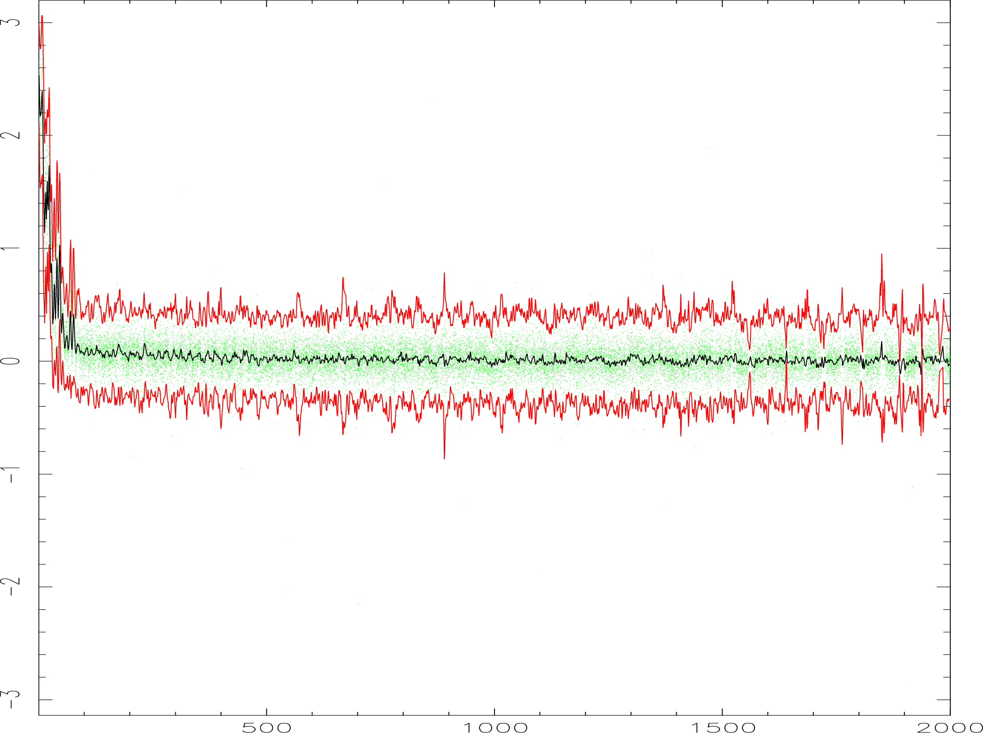
XRANGE - X range of plot (! to continue) /[1,5112]/ > 1,2000
XRANGE - X range of plot (! to continue) /[1,2000]/ > !
SURF: 8 spikes detected in file hl39_lon_sky
...........................
SURF: 196 spikes detected in file hl42_lon_sky
OUT - Name of despiked data file /’hl39_lon_dsp’/ >
...........................
OUT - Name of despiked data file /’hl42_lon_dsp’/ >
The display for the first 2000 data points are shown in Fig. 7. Note that after you run despike the
display may get messed up. It is normally sufficient to clear the display with gdclear and re-issue the
the color table, e.g. lutbgyrw. If there are still problems, delete the AGI-file from your home directory
(agi_xxx.sdf, where xxx is the name of your work station).
We now run rebin on each data set to determine the offsets we need to center the map, which will
ensure that we get the sharpest possible image. We also determine the rms noise level for each map.
Here it is a clear advantage to use Gaia. After displaying the map with your preferred color
scheme and contrast level using the View menu, go to the Image-Analysis menu and click
on image regions. Choose the polygon option of ARD regions and outline the region you
want to use with the cursor. After it is done, click on Stats selected and you are done. For
determining pointing offsets it is easier to use the Kappa command centroid i.e. centroid
search=19 cerror, where we adjust the search parameter to minimize the fit errors. For
850 m
and a 1 arcsec cell setting search to 17 or 19 generally gives a good result. After we have
determined the noise level and position offsets for each map we compute the weights for
each map. An easy way to do this is to set the weight for the first map equal to one. All
other maps are then weighted relative to this map. If we call the integration times
t and
t, and the corresponding
noise values n
and n
for map 1 and map 2 respectively, then we can compute the weighting factor from the following
equation:
|
| (3) |
We now edit in the weights and position offset in hl.inp and run despike again on the original data
set. The end result appears good enough.
Now we can form the final co-add of the data very easily, since we have already computed the
weights and position shifts that we need to get the best S/N and sharpest image from our data. The
only thing we need to do is to change the file extensions from sky to dsp, the name we used for
despiked data files. We rename the input file to hl.dsp in case we would like to redo the despiking.
We now run this file through rebin, i.e.,
% rebin noloop
REBIN_METHOD - Rebinning method to be used /’LINEAR’/ >
SURF: Initializing LINEAR weighting functions
OUT_COORDS - Coordinate sys of output map; PL,AZ,NA,RB,RJ,RD or GA
/’RJ’/ >
SURF: output coordinates are FK5 J2000.0
REF - Name of first data file to be rebinned /’hl42_lon_dsp’/ >
hl.inp
SURF: Reading file hl39_lon_dsp
SURF: run 39 was a MAP observation of HLTau with JIGGLE sampling
SURF: file contains data for 4 exposure(s) in 3 integrations(s) in 1
measurement(s)
..................
SURF: Reading file hl42_lon_dsp
SURF: run 42 was a MAP observation of HLTau with JIGGLE sampling
SURF: file contains data for 4 exposure(s) in 3 integrations(s) in 1
measurement(s)
SURF Input data: (name, weight, dx, dy)
-- 1: hl39_lon_dsp (1, 0.08, 1.19)
-- 2: hl64_lon_dsp (0.4, 0.64, 0.75)
-- 3: hl41_lon_dsp (0.9, -0.23, 2.7)
-- 4: hl55_lon_dsp (1, -0.86, 0.38)
-- 5: hl61_lon_dsp (0.8, 0.14, 1.04)
-- 6: hl75_lon_dsp (0.75, 0.4, -0.13)
-- 7: hl84_lon_dsp (0.5, 0.42, 0.83)
-- 8: hl60_lon_dsp (0.9, 0.11, -1.41)
-- 9: hl23_lon_dsp (0.75, 0.1, 0.46)
-- 10: hl42_lon_dsp (0.3, 0.75, 1.06)
LONG_OUT - Longitude of of output map centre in hh (or dd) mm ss.ss
format
/’+04 31 38.46’/ >
LAT_OUT - Latitude of output map centre in dd mm ss.ss format
/’+ 18 13 57.8’/ >
OUT_OBJECT - Object name for output map /’HLTau’/ >
PIXSIZE_OUT - Size of pixels in output map (arcsec) /3/ > 1
SIZE - Number of pixels in output map (NX,NY) /[194,192]/ >
OUT - Name of file to contain rebinned map /’HLTau’/ > hltau_lon
WTFN_REGRID: Beginning regrid process
WTFN_REGRID: Entering second rebin phase (T = 3.113513 seconds)
WTFN_REGRID: Entering third rebin phase (T = 14.55025 seconds)
WTFN_REGRID: Regrid complete. Elapsed time = 15.23921 seconds
We now have our final co-added map, which is almost as good as it can get from the data we had
available.
If you have extremely large data sets, then you may find that your computer runs out of memory in
rebin. The recommended solution, if you cannot find a more powerful workstation, is to split the data
set in two parts, run each separately through rebin, and co-add the two final maps using the
Kappa command add or the task makemos in Ccdpack.