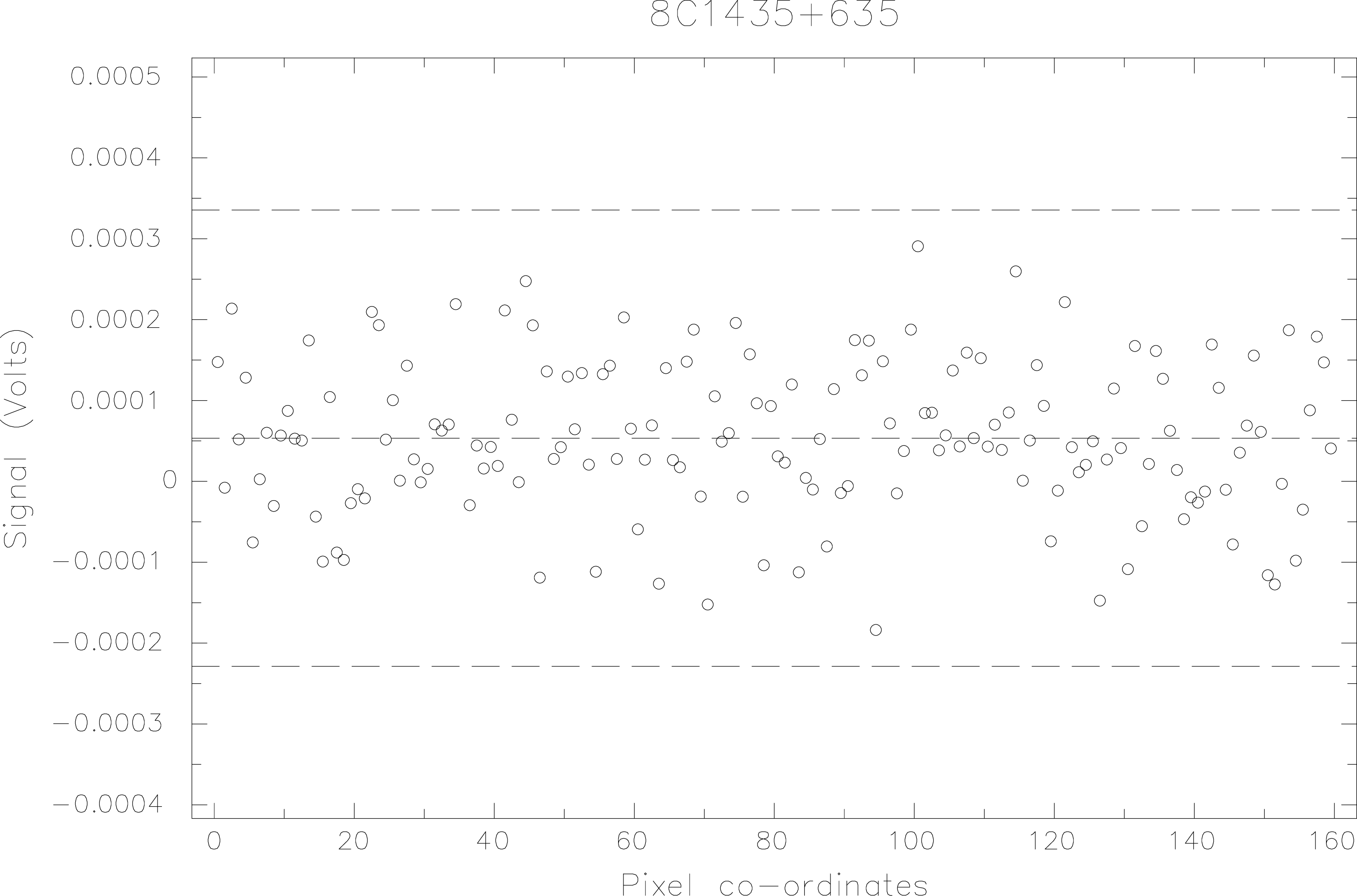
Figure 4: A 48 minute (160 x 9/2.0 jiggle patterns) integration on 8C1435+635.
The sigclip command has been used to produce a dataset despiked at the
3
level.
Photometric observations of faint sources often require that the source be observed for long periods, during which the atmospheric conditions and/or telescope related parameters such as pointing and focus may vary. These effects are particularly noticeable around sunrise and sunset, for example. The consistency of the entire data set can be investigated with the use of a two sample Kolmogorov-Smirnov (KS) test. Again, the method adopted for the SCUBA data reduction package is analogous to that used previously by COADD for UKT14 [7].
The data set is split into subsamples that are specified by the user. The size of these subsamples clearly depends on the total number of photometric points and some experimentation is required but, for example, if the data set consists of 100 points then subsamples of 20 would be a sensible choice. The first subsample is compared with the second and is ‘rejected’ if the probability that the two are statistically different is lower than a user specified tolerance. If the KS test returns 0.1 then this indicates that there is a 90% probability that the two samples are different. If the first two subsamples are consistent then they are concatenated and compared with the third etc, otherwise the first subsample is compared with the third and so on. A problem arises if, for some reason, the first subsample is different from each of the others since in this case most of the data set will be rejected. If this happens it is necessary to repeat the process but this time select a different subsample against which the others are to be compared. In general, it is good practice to change the order and repeat the test.
The best way to illustrate the whole process is with an example using real data.
For the example I’ll use the 8C1435+635 measurement at 850m that was discussed in §4.2. Here the whole data set has been reduced with sky removal, concatenated and despiked using sigclip (see Figure 4). Note that sigclip must be used rather than drawsig because it produces an output file devoid of spikes. I renamed this file 8c_clip for brevity.
The kstest command is part of the Starlink Kappa package and takes a variety of parameters. In this document I’ll just discuss those relevant to the basic KS test as applicable to photometry data. A full description of the routine can be found in the Kappa manual (SUN/95).
I’ll split the dataset into subsamples of 20 integrations (the second subsample will contain only 19 points because sigclip removed one spike). In this example, the input and output file names are specified on the command line but this need not be the case. Note that it is, however, necessary to give the number of samples and the probability in the same way, otherwise the default values of 3 and 0.05 are assumed respectively. A maximum number of 20 subsamples is allowed by kstest.
Subsample 6 which contains many more points with a signal greater than zero compared to the other subsamples is rejected (see Figure 4). If you wish to view the truncated dataset then 8c_ks.sdf can be displayed with qdraw in the usual way.
If the first sample is anomalous then we can repeat the test in reverse order by applying the Kappa command flip to the original dataset, 8c_clip;
More generally, any subsample can be specified with a NDF section [8]. In the above example, subsample 7 is 8c_clip(121:140). The kstest command can then read in an ascii file containing a list of NDF sections, such as,
The following command then performs the KS test using this file;
NSAMPLE parameter is now redundant and also that single quotes must surround the
input file name. The final result in this case is unchanged, of course.