5 Sample reductions

 5.1 Example reduction – long method
 5.2 Example reduction - scuquick

The following two sections show sample reductions of real photometric data, first by the long winded method of typing each of the Surf commands in turn and then using the perl [6] script scuquick which provides some level of automation.

For the first example, I’ll use two 20 integration observations of the radio galaxy 3C 31 which were made at 2.0 mm during the astronomical commissioning on a poor night (the zenith optical depth at 225 GHz was about 0.1). I’ll use change_flat to change the flatfield file although, since we are using one of the photometric pixels, flatfielding is not necessary.

5.1 Example reduction – long method

The first observation is #70:

  % reduce_switch
  IN - Name of input file containing demodulated data > 19970807_0070
  USE_CALIBRATOR - Should the data be divided by the internal calibrator /NO/ >
  SURF: run 70 was a PHOTOM observation of object 3C31
  SURF: file contains data for 2 switch(es) in 1 exposure(s) in 20 integration(s)
  in 1 measurement(s)
  SPIKE_LEVEL - De-spike level /5/ >
  OUT - Name of output file to contain reduced switch data > red70
  % change_flat
  IN - Name of input file containing demodulated map data /@red70/ >
  SURF: run 70 was a PHOTOM observation of 3C31
  NEW_FLAT - The name of the file containing the new flat-field > noiseflat.dat
  % flatfield
  IN - Name of input file /@red70/ >
  SURF: run 70 was a PHOTOM observation of 3C31
  OUT - Name of output file > red70_flat
  SURF: applying flatfield from noiseflat.dat
  % extinction
  IN - Name of NDF containing demodulated data /@red70_flat/ >
  SURF: run 70 was a PHOTOM observation with JIGGLE sampling of object 3C31
  SURF: file contains data for 1 exposure(s) in 20 integration(s) in 1
  measurement(s)
  SURF: observation started at sidereal time 2 35 59.4417688 and ended at 2 52
  07.164001
  SURF: file contains data for the following sub-instrument(s)
   - P2000 with filter 2000
  FIRST_TAU - First zenith sky opacity measured > 0.1
  FIRST_LST - Sidereal time of first opacity measurement; hh mm ss.ss > 0
  SECOND_TAU - Second zenith sky opacity measured > 0.1
  SECOND_LST - Sidereal time of second opacity measurement; hh mm ss.ss > 0
  OUT - Name of output NDF > red70_ext
  % scuphot
  IN - Name of input file containing demodulated data /@red70_ext/ >
  SURF: run 70 was a PHOTOM observation of 3C31
  SURF: file contains data for 1 exposure(s) in 20 integrations(s) in 1
  measurement(s)
  ANALYSIS - Which reduction method /’AVERAGE’/ >
  OUT - Name of container file to hold map and time-sequence data > red70_phot
  FILE - Name of ASCII file to contain results summary // > red70_phot.dat

The ASCII file, red70_phot.dat, contains the following:

  % cat red70_phot.dat
  Output from REDS reduction of a PHOTOM observation
  Reduction date        : Mon May 19 12:04:08 1997
  Observation definition: 3c31.obs
  Date of observation   : 1996:8:7
  Time of observation   : 15:52:07.659988
  Run number            : 70
  Object                : 3C31
  Sub-instrument        : P2000
  Filter                : 2000
  Centre coords         : RB
  Latitude              : +32:08:43.3
  Longitude             : 01:04:39.10
  Offset coords         : UNKNOWN
  x offset              : 0
  y offset              : 0
  Sample coords         : NA
  Sky error removal     : FALSE
  
  Photometric analysis  : AVERAGE
  
  Bolometer: G6
  Weight:    1
  
  Integration  Peak    Error       S/N      Peak_x     Peak_y
     1    0.294E-04  0.461E-02    0.006  0.000E+00  0.000E+00
     2    0.146E-03  0.461E-02    0.032  0.000E+00  0.000E+00
     3    0.168E-03  0.460E-02    0.036  0.000E+00  0.000E+00
     4    0.174E-03  0.461E-02    0.038  0.000E+00  0.000E+00
     5    0.103E-03  0.459E-02    0.023  0.000E+00  0.000E+00
     6    0.116E-03  0.460E-02    0.025  0.000E+00  0.000E+00
     7    0.182E-03  0.461E-02    0.039  0.000E+00  0.000E+00
     8    0.321E-04  0.462E-02    0.007  0.000E+00  0.000E+00
     9    0.959E-04  0.462E-02    0.021  0.000E+00  0.000E+00
    10   -0.481E-03  0.466E-02   -0.103  0.000E+00  0.000E+00
    11    0.705E-04  0.466E-02    0.015  0.000E+00  0.000E+00
    12    0.445E-04  0.496E-02    0.009  0.000E+00  0.000E+00
    13    0.640E-04  0.468E-02    0.014  0.000E+00  0.000E+00
    14    0.490E-04  0.470E-02    0.010  0.000E+00  0.000E+00
    15    0.272E-03  0.469E-02    0.058  0.000E+00  0.000E+00
    16    0.170E-03  0.471E-02    0.036  0.000E+00  0.000E+00
    17    0.174E-03  0.471E-02    0.037  0.000E+00  0.000E+00
    18    0.149E-03  0.473E-02    0.032  0.000E+00  0.000E+00
    19   -0.609E-04  0.474E-02   -0.013  0.000E+00  0.000E+00
    20   -0.874E-03  0.480E-02   -0.182  0.000E+00  0.000E+00
  
  Measurement results:
   Parabolic fit to coadded jiggle:
          0.105E-03  0.385E-04    2.713 -0.170E+01  0.299E+00
    Coadded result of individual integrations:
          0.312E-04  0.584E-04    0.534


pdfpict

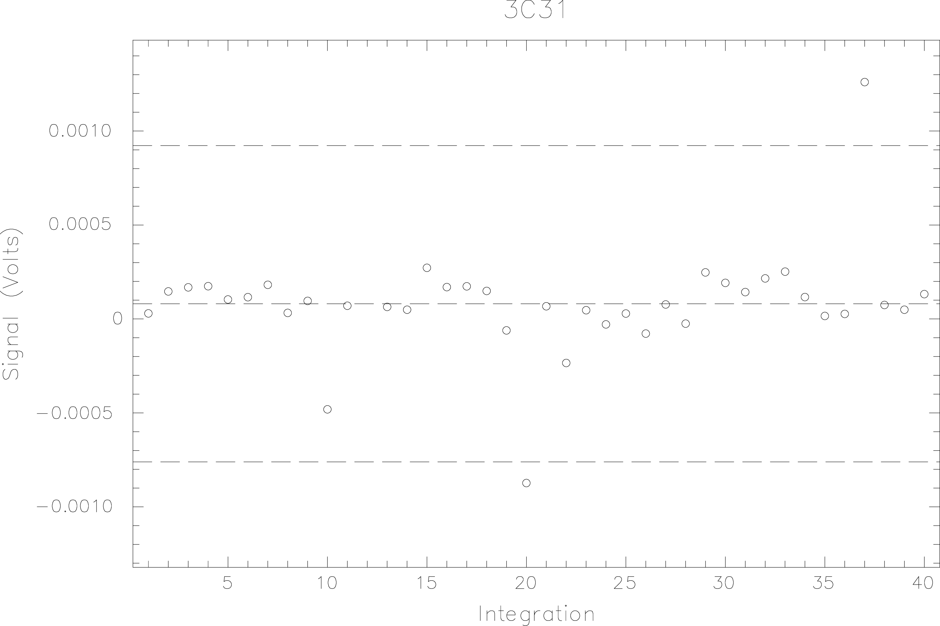
Figure 1: Concatenated data for observations #70 and #71. The mean and plus and minus 3σ levels are indicated with the dashed lines.


The same procedure is repeated (not shown here) for #71 to produce the file red71phot.sdf. We can then combine the two observations using scucat:

  % scucat
  OUT - Rootname of files to contain concatenated data > 3C31_2000
  IN - Name of input file containing photometry data > red70_phot
  SURF: Found data for the following bolometers: g6
  SURF: This is a PHOTOM observation of 3C31. There are 20 integrations
  IN - Name of input file containing photometry data /!/ > red71_phot
  SURF: Found data for the following bolometers: g6
  SURF: This is a PHOTOM observation of 3C31. There are 20 integrations
  IN - Name of input file containing photometry data /!/ >

We are now in a position to plot and despike the data (see Figure 1). Note that the bolometer name, g6, will be appended to the file name giving 3C31_2000_g6.sdf.

  % qdraw 3C31_2000_g6 mode=4 device=xwindows
  NDF is 3C31_2000_g6
  The default values have been adopted for parameter ABSLIM.
  Current picture has name: DATA, comment: KAPPA_LINPLOT.
  Using /home/jas/scuba/test/3C31_2000_g6 as the input NDF.
  
        Clip (+/-)         mean          std. deviation    Error in mean
        ----------         ----          --------------    -------------
                        0.800321E-04      0.276960E-03      0.437913E-04
           3.000        0.740715E-04      0.136353E-03      0.221194E-04

Clearly, this data set contains large spikes and the best despiking strategy is to remove the two biggest spikes that fall outside the 3σ levels and then replot the data. For this we use the sigclip command.


pdfpict

Figure 2: Concatenated data for #70 and #71 after removal of the two largest spikes with 
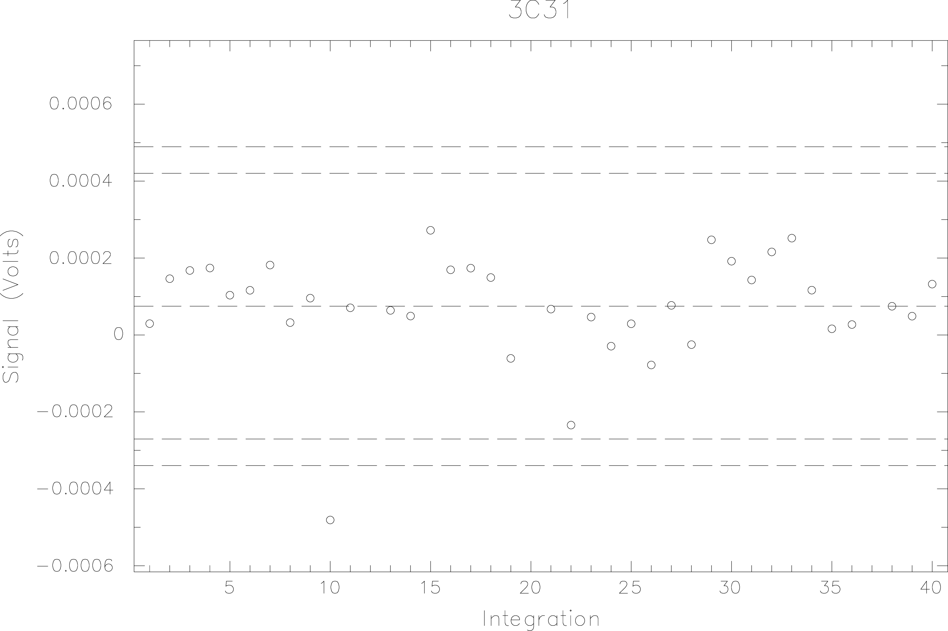
sigclip. The third spike is now excluded with a 3σ clip and there are no further spikes at the 2.5σ level.


  %  sigclip 3C31_2000_g6 3.0
  There was 1 element changed in the DATA array below the threshold.
  There was 1 element changed in the DATA array above the threshold.
  Clipped data written to 3C31_2000_g6_clip.sdf
  %  qdraw 3C31_2000_g6_clip device=xwindows mode=4
  NDF is 3C31_2000_g6_clip
  The default values have been adopted for parameter ABSLIM.
  Current picture has name: DATA, comment: KAPPA_LINPLOT.
  Using /home/jas/scuba/test/3C31_2000_g6_clip as the input NDF.
  
        Clip (+/-)         mean          std. deviation    Error in mean
        ----------         ----          --------------    -------------
                        0.740715E-04      0.136353E-03      0.221194E-04
           3.000        0.890766E-04      0.101563E-03      0.166969E-04
  %
  %  drawsig nsigma=2.5 device=xwindows
  Current picture has name: DATA, comment: KAPPA_LINPLOT.
  Using /home/jas/scuba/test/3C31_2000_g6_clip as the input NDF.
  
        Clip (+/-)         mean          std. deviation    Error in mean
        ----------         ----          --------------    -------------
                        0.740715E-04      0.136353E-03      0.221194E-04
           2.500        0.890766E-04      0.101563E-03      0.166969E-04

All three obvious spikes have now been removed and there are no further spikes down to the 2.5-σ level (see Figure 2). The source is detected at the 5.3-σ level.

5.2 Example reduction - scuquick

The PERL script scuquick can be used to save time by automating the reduction process up to and including the scuphot stage. Note that if many repetitive operations are to be performed then scuquick (or any other Surf command) will take options. For example,

  % scuquick -remsky

will invoke the remsky command at the appropriate position in the reduction process. A list of avialable options can be accessed by typing

  % scuquick -h
  
  Usage:
     scuquick [-h] [-change_flat] [-remsky] [-rebin] [-notau|tau f] [-sub s]
  Options:
     -h[elp]       This message
     -quick        Run all tasks with the ’accept’ flag (ie take defaults)
     -quiet        Hide all messages generated by the script (note this is
                   not the same as using MSG_FILTER=quiet which hides messages
                   from the tasks)
     -change_flat  Run the change_flatfield task
     -remsky       Run remsky
     -rebin        Regrid the data
     -sub s        Select a specific sub-instrument (else selects all)
     -notau        Use a tau value of 0 in extinction
     -tau f        Use a constant value (f) for the tau. This is dangerous
                   when reducing data containing multiple sub-instruments
                   unless the -sub flag is used.
  
  Notes:
     Parameters for any task can be specified on the command line
     as param=value. All other command line arguments are assumed to be
     input NDFs.

The second example uses scuquick to reduce a long integration on the radio galaxy 8C1435+635 at 450 and 850μm. Note that scuquick will reduce data from both arrays unless instructed otherwise by use of the -sub option.

This data set was obtained under moderately noisy sky conditions so sky removal will be used in an attempt to correct for the sky variations. I’ll just reduce the first demodulated data file here.

  % scuquick -remsky
  IN - Name of input file containing demodulated data > 19970502_dem_0052
  SURF: run 52 was a PHOTOM observation of object 8C1435+635
  USE_CALIBRATOR - Should the data be divided by the internal calibrator /NO/ >
  SURF: file contains data for 2 switch(es) in 1 exposure(s) in 40 integration(s)
  in 1 measurement(s)
  SPIKE_LEVEL - De-spike level /5/ >
  OUT - Name of output file to contain reduced switch data > r52
  SURF: run 52 was a PHOTOM observation of 8C1435+635
  SURF: applying flatfield from photflat1.dat
  
  Processing the LONG sub instrument
  
  SURF: run 52 was a PHOTOM observation with JIGGLE sampling of object 8C1435+635
  SURF: file contains data for 1 exposure(s) in 40 integration(s) in 1
  measurement(s)
  SURF: observation started at sidereal time 14 54 12.45781 and ended at 15 14
  46.826715
  SURF: file contains data for the following sub-instrument(s)
   - LONG with filter 850
   - SHORT with filter 450
  FIRST_TAU - First zenith sky opacity measured > 0.18
  FIRST_LST - Sidereal time of first opacity measurement; hh mm ss.ss > 0
  SECOND_TAU - Second zenith sky opacity measured > 0.18
  SECOND_LST - Sidereal time of second opacity measurement; hh mm ss.ss > 0
  Extinction corrected data has been written to file r52_ext_long.sdf
  SURF: run 52 was a PHOTOM observation with JIGGLE sampling of object 8C1435+635
  BOLOMETERS - The Sky bolometers, [a1,a2] for an array /[’d10’,’c16’,’c12’,
  ’c2’,’b9’,’b10’,’b11’,’c5’,’c16’,’d10’,’e2’,’e3’]/ > [h6,h8,h13,h14,g15,g16]
  MODE - Sky removal mode /’MEAN’/ >
  ITER_SIGMA - Sigma level to drop points from mean iteratively /-1/ > 3.
  CLIP - Do you wish to clip the bolometers? /NO/ >
  Sky corrected data has been written to file r52_sky_long.sdf
  SURF: run 52 was a PHOTOM observation of 8C1435+635
  SURF: file contains data for 1 exposure(s) in 40 integrations(s) in 1
  measurement(s)
  ANALYSIS - Which reduction method /’AVERAGE’/ >
  Processed photometry data written to r52_phot_long.sdf and r52_phot_long.dat
  
  Processing the SHORT sub instrument
  
  SURF: run 52 was a PHOTOM observation with JIGGLE sampling of object 8C1435+635
  SURF: file contains data for 1 exposure(s) in 40 integration(s) in 1
  measurement(s)
  SURF: observation started at sidereal time 14 54 12.45781 and ended at 15 14
  46.826715
  SURF: file contains data for the following sub-instrument(s)
   - LONG with filter 850
   - SHORT with filter 450
  FIRST_TAU - First zenith sky opacity measured > 1.0
  FIRST_LST - Sidereal time of first opacity measurement; hh mm ss.ss > 0
  SECOND_TAU - Second zenith sky opacity measured > 1.0
  SECOND_LST - Sidereal time of second opacity measurement; hh mm ss.ss > 0
  Extinction corrected data has been written to file r52_ext_short.sdf
  SURF: run 52 was a PHOTOM observation with JIGGLE sampling of object 8C1435+635
  BOLOMETERS - The Sky bolometers, [a1,a2] for an array /[’h6’,’h8’,’h13’,’h14’,
  ’g15’,’g16’]/ > [d10,c16,c12,c2,b9,b10,b11,c5,c16,d10,e2,e3]
  MODE - Sky removal mode /’MEAN’/ >
  ITER_SIGMA - Sigma level to drop points from mean iteratively /-1/ > 3.
  CLIP - Do you wish to clip the bolometers? /NO/ >
  Sky corrected data has been written to file r52_sky_short.sdf
  SURF: run 52 was a PHOTOM observation of 8C1435+635
  SURF: file contains data for 1 exposure(s) in 40 integrations(s) in 1
  measurement(s)
  ANALYSIS - Which reduction method /’AVERAGE’/ >
  Processed photometry data written to r52_phot_short.sdf and r52_phot_short.dat

and similarly for the rest of the data after which scucat and display/despike procedures can be followed as before. Note that I took the ‘default’ sky bolometers which correspond to the inner ring of the long-wave array in this case - in fact these are not strictly the default but rather the last combination that were used. I recommend reducing the data both with and without sky removal since under very stable conditions the signal-to-noise can be degraded by removing the sky. A useful aid is a plot of signals from the source bolometer and sky removal bolometers. There are a variety of ways of doing this: Appendix A describes how to get ascii output for any bolometer; here I’ll use Surf and Kappa commands to investigate the effects of the adopted sky removal. Firstly, we can use scuphot and scucat to write out data for all bolometers in a file - in this case observation #52 as before. I’ll use the extinction corrected data because these have been processed by flatfield;

  % scuphot allbols=true
  IN - Name of input file containing demodulated data // > r52_ext_long
  SURF: run 52 was a PHOTOM observation of 8C1435+635
  SURF: file contains data for 1 exposure(s) in 40 integrations(s) in 1
  measurement(s)
  ANALYSIS - Which reduction method /’AVERAGE’/ >
  OUT - Name of container file to hold map and time-sequence data > r52_all
  SCUPHOT: All bolometers selected
  FILE - Name of ASCII file to contain results summary /!/ > r52_all.dat
  % scucat
  OUT - Rootname of files to contain concatenated data > r52
  IN - Name of input file containing photometry data // > r52_all
  SURF: Found data for the following bolometers:
  g1,g2,g3,g4,g7,g8,g9,g10,g11,g13,g14,g15,g16,h1,h2,h4,h5,h6,h7,h8,h9,h10,h11,h1
  2,h13,h14,h15,h16,i1,i2,i3,i4,i5,i6,i7,i8,i9
  SURF: This is a PHOTOM observation of 8C1435+635. There are 40 integrations
  IN - Name of input file containing photometry data /!/ >

Each bolometer now has a file called, e.g. r52_h7.sdf. The Kappa commands add and cdiv can be used to get a mean sky value for the inner ring.


pdfpict

Figure 3: Comparison of the the signal from the central bolometer of the long-wave array with the mean signal from the six surrounding sky bolometers. Correlated sky noise is clearly seen in this case.


  % add
  IN1 - First input NDF /’r52_all’/ > r52_h6
  IN2 - Second input NDF > r52_h8
  OUT - Output NDF > sum
  % add
  IN1 - First input NDF /@sum/ > sum
  IN2 - Second input NDF > r52_h13
  OUT - Output NDF > sum1
  % add
  IN1 - First input NDF /@sum1/ > sum1
  IN2 - Second input NDF > r52_h14
  OUT - Output NDF > sum2
  % add
  IN1 - First input NDF /@sum2/ >
  IN2 - Second input NDF > r52_g15
  OUT - Output NDF > sum3
  % add
  IN1 - First input NDF /sum3/ >
  IN2 - Second input NDF > r52_g16
  OUT - Output NDF > sum4
  % cdiv
  IN - Input NDF data structure /@sum4/ >
  SCALAR - Division constant /6/ >
  OUT - Output NDF > inner_ring
  %

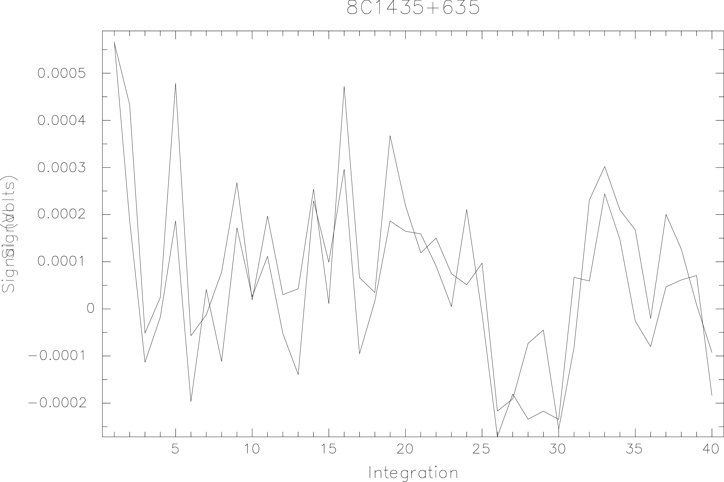
and then use linplot to overlay the data (you can use e.g. lincol=red to get coloured plots),

  % linplot r52_h7 device=xwindows mode=line
  % linplot inner_ring device=xwindows mode=line noclear

Figure 3 shows the output from linplot which clearly shows that the signal and sky are correlated in this case.