11 Calculating Statistics

In the same way that it was useful to display images at intermediate stages in the data reduction, it is often useful to be able to calculate and list gross statistics (mean value, standard deviation etc.) for images as they are processed. There are a couple of applications which provide this facility. Proceed as follows.

(1)
Assuming that KAPPA is loaded (see the recipe in Section 9), move to the subdirectory containing the target astronomical images and type:
  % stats ngc2336_r_2

The following information should be displayed:

  Pixel statistics for the NDF structure /acdscratch/sc5/targets/ngc2336_r_2
  
     Title                     : N2366 R
     NDF array analysed        : DATA
  
        Pixel sum              : 1.6012529E9
        Pixel mean             : 1267.44
        Standard deviation     : 279.5582
        Minimum pixel value    : 166
           At pixel            : (1, 547)
           Co-ordinate         : (0.5, 546.5)
        Maximum pixel value    : 50963
           At pixel            : (1023, 146)
           Co-ordinate         : (1022.5, 145.5)
        Total number of pixels : 1263376
        Number of pixels used  : 1263376 (100.0%)

(2)
The statistics can also be written to a log file. Type:
  % stats ngc2336_r_2 logfile=ngc2336_r_2.log

Text file ngc2336_r_2.log will be created containing a copy of the output.

(3)
stats has a ‘κ-sigma clipping’ option which allows outlying values, such as star images, to be rejected when computing the statistics. If a clipping level is given, stats will compute statistics using all the available pixels, reject all those pixels whose values lie outside κ standard deviations of the mean and then re-evaluate the statistics. An array of up to five clipping levels may be given, which are applied sequentially. For example, to reject values outside two standard deviations type:
  % stats ngc2336_r_2 clip=2

The statistics will again be displayed, but this time the clipping will have been applied before they were computed.

(4)
Often the information generated by stats will be adequate. However, application histpeak in the ESP package (see SUN/180[12]) gives further details. To load ESP type:
  % esp

then type histpeak and respond to the prompts:

  % histpeak
  
  ESP HISTPEAK running.
  
  IN - Image NDF filename /@ngc2336_r_2/ > ngc2336_r_2
  Filename:   /acdscratch/sc5/targets/ngc2336_r_2
  Title:      N2366 R
  Shape:      1124 x 1124  pixels
  Bounds:     x = 1:1124  y = 1:1124
  Image size: 1263376 pixels
  
  USE - Use the whole image or an ARD file /’w’/ >
  
  SFACT - Smoothing width you wish to use /0/ >
  
  DEVICE - Display device code or name /@xwindows/ >

Output similar to the following should be produced:

  HISTPEAK Results: /acdscratch/sc5/targets/ngc2336_r_2
  
  Pixels (used):            1263376     Pixels (bad):                0
  Lowest count:             166.000     Highest count:       50963.000
  Skewness:                  63.680     Kurtosis:             7114.975
  
  Mean:                    1267.440     Median:               1294.776
  
  Histogram modal values:
  Unsmoothed:              1298.000     Smoothed:             1298.000
  Projected:               1296.511     Interpolated:         1298.696
  
  Absolute dev.:             90.361     Variance:               78153.
  Standard. dev.:           279.558     Back. st. dev.:         33.353
  
  Smoothing filter radius:
  Radius request:                 0     Radius actual:               0
  
  Contents of the most occupied histogram bin:
  Unsmoothed:             21104.000     Smoothed:            21104.000
  Interpolated:           12126.075

and a plot similar to Figure 11 should appear. For the purpose of determining the sky background level it is probably best to use either histpeak or stats with the clipping option. Also note that the histpeak pre-amble contains the dimensions and bounds of the image.


pdfpict

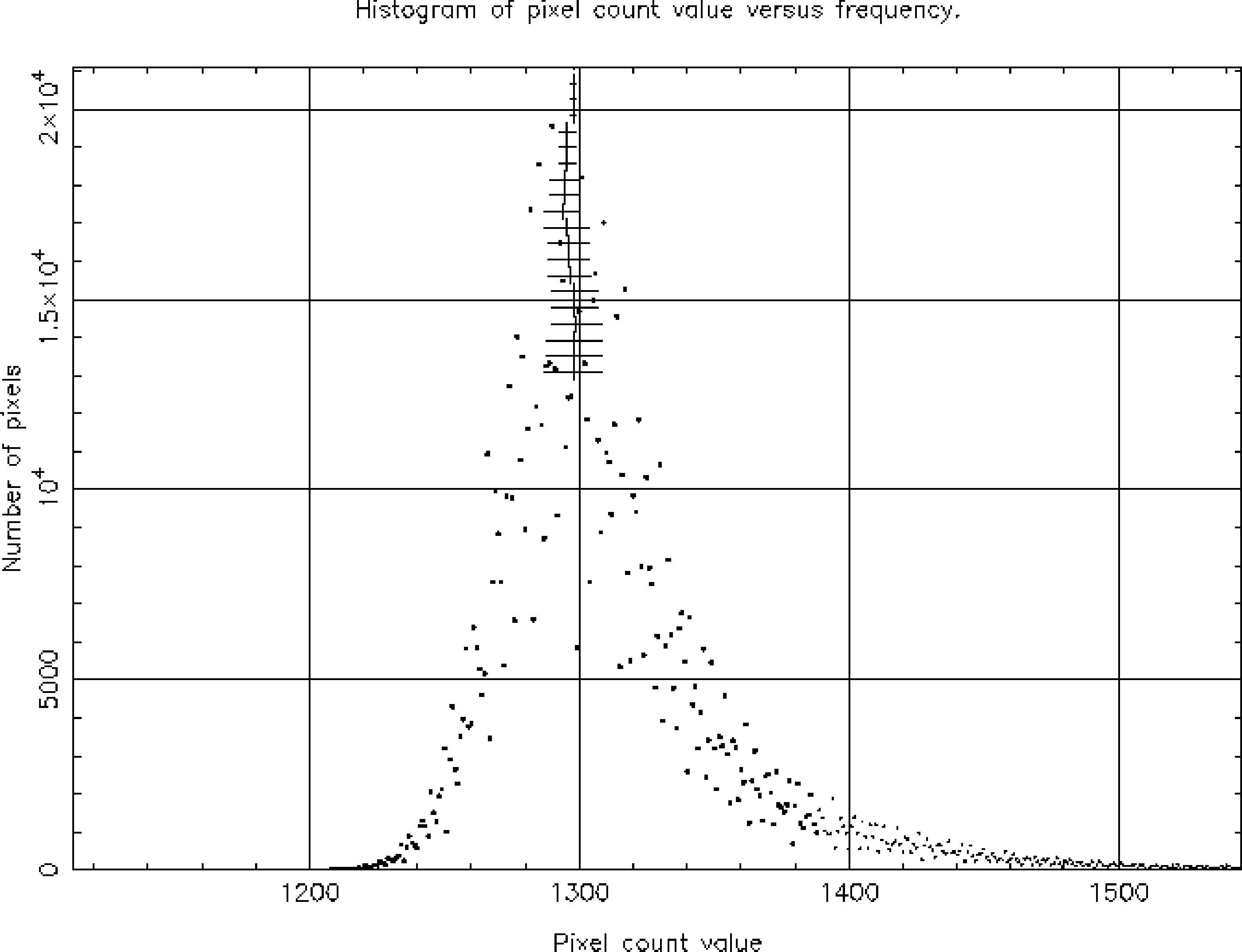
Figure 11: Example of histogram produced by histpeak